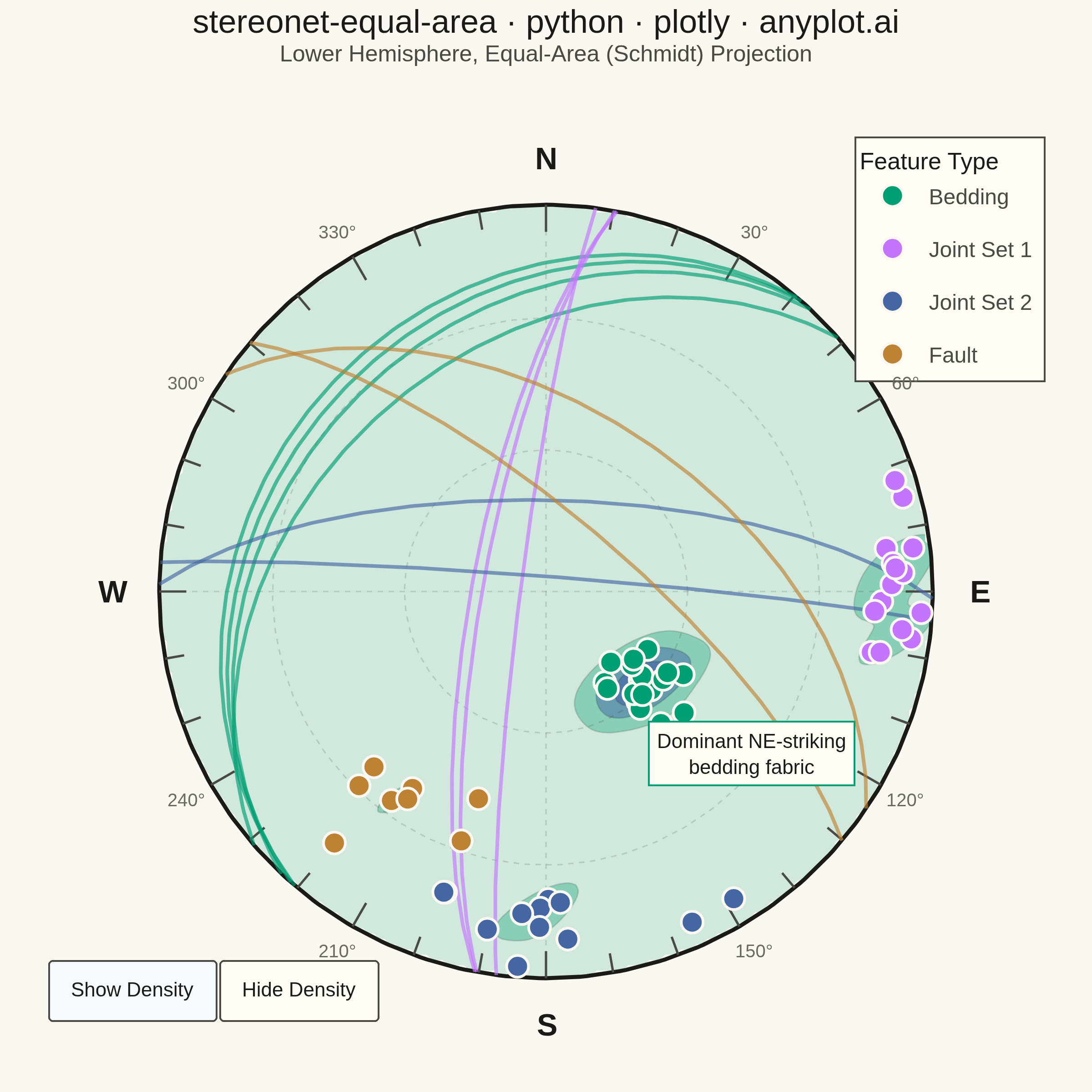
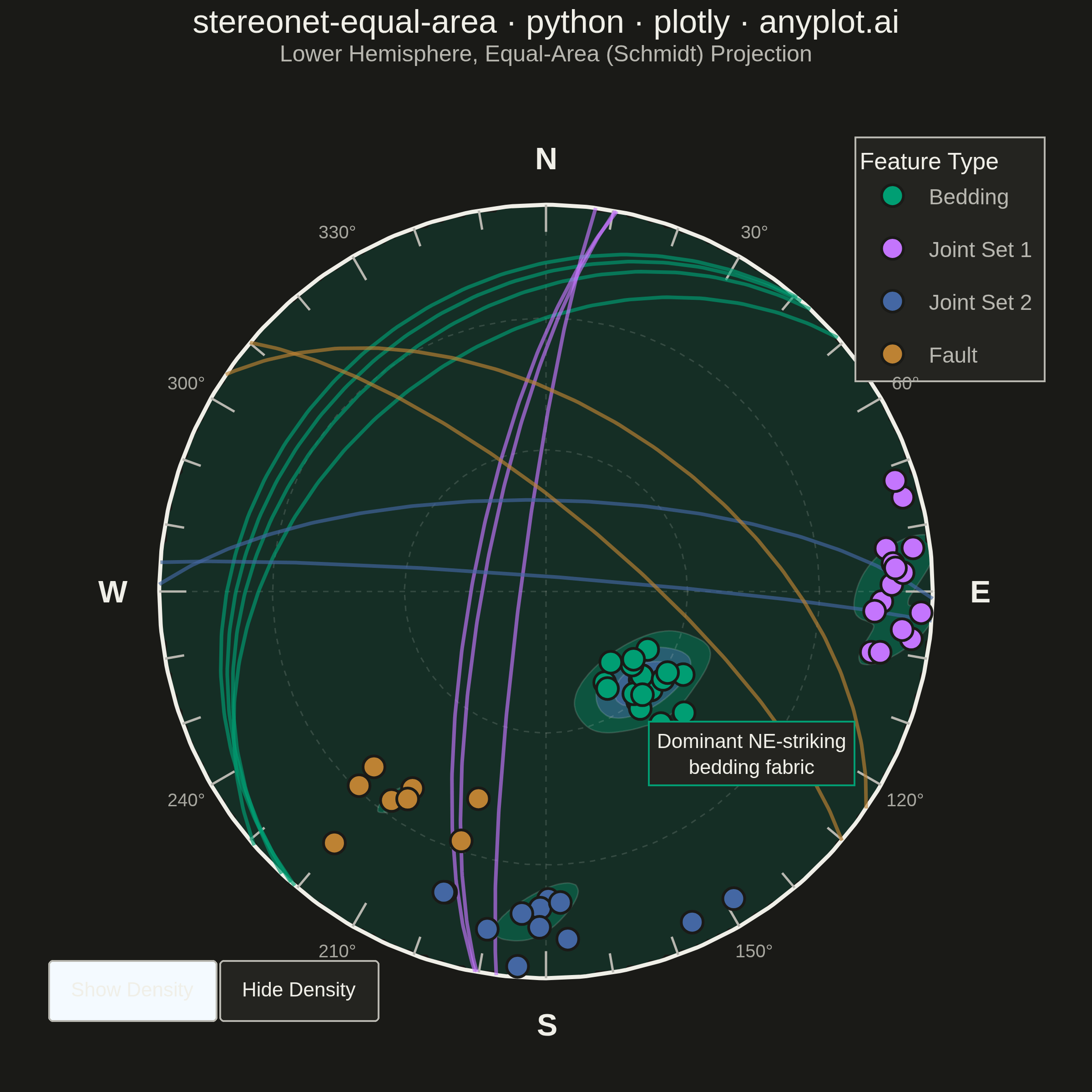
A Schmidt equal-area (lower-hemisphere) stereographic projection for plotting geological structural data. Great circles represent planar features (bedding, faults, joints) by their strike and dip, while poles to planes are plotted as points showing the orientation of the normal to each plane. Density contours highlight preferred orientations in clustered data. This is the standard projection used in structural geology for analyzing fabric elements and kinematic indicators.
""" anyplot.ai
stereonet-equal-area: Structural Geology Stereonet (Equal-Area Projection)
Library: plotly 6.8.0 | Python 3.13.13
Quality: 92/100 | Updated: 2026-06-16
"""

import os

import numpy as np
import plotly.graph_objects as go
from scipy.stats import gaussian_kde


# Theme-adaptive chrome (Imprint palette)
THEME = os.getenv("ANYPLOT_THEME", "light")
PAGE_BG = "#FAF8F1" if THEME == "light" else "#1A1A17"
ELEVATED_BG = "#FFFDF6" if THEME == "light" else "#242420"
INK = "#1A1A17" if THEME == "light" else "#F0EFE8"
INK_SOFT = "#4A4A44" if THEME == "light" else "#B8B7B0"
INK_MUTED = "#6B6A63" if THEME == "light" else "#A8A79F"
RULE = "rgba(26,26,23,0.15)" if THEME == "light" else "rgba(240,239,232,0.15)"

# Imprint categorical palette — feature types are abstract, so canonical order.
# Bedding takes the brand green (always-first series).
IMPRINT_PALETTE = ["#009E73", "#C475FD", "#4467A3", "#BD8233"]

# Data - Field measurements from a structural geology mapping campaign
np.random.seed(42)

# Bedding planes: NE-striking, moderate SE dip
bedding_strike = np.random.normal(45, 8, 20)
bedding_dip = np.random.normal(30, 5, 20)

# Joint set 1: N-S striking, steep E dip
joint1_strike = np.random.normal(0, 10, 15)
joint1_dip = np.random.normal(80, 5, 15)

# Joint set 2: E-W striking, steep S dip
joint2_strike = np.random.normal(90, 12, 12)
joint2_dip = np.random.normal(75, 8, 12)

# Faults: NW-SE striking, moderate dip
fault_strike = np.random.normal(130, 15, 8)
fault_dip = np.random.normal(55, 10, 8)

strikes = np.concatenate([bedding_strike, joint1_strike, joint2_strike, fault_strike])
dips = np.concatenate([bedding_dip, joint1_dip, joint2_dip, fault_dip])
feature_types = ["Bedding"] * 20 + ["Joint Set 1"] * 15 + ["Joint Set 2"] * 12 + ["Fault"] * 8
strikes = strikes % 360
dips = np.clip(dips, 0, 90)

type_colors = {
    "Bedding": IMPRINT_PALETTE[0],
    "Joint Set 1": IMPRINT_PALETTE[1],
    "Joint Set 2": IMPRINT_PALETTE[2],
    "Fault": IMPRINT_PALETTE[3],
}

# Equal-area (Schmidt) projection of poles to planes
# Pole to plane: trend = dip direction = strike + 90°, plunge = 90° - dip
pole_trend_rad = np.radians((strikes + 90) % 360)
pole_plunge_rad = np.radians(90 - dips)
pole_r = np.sqrt(2) * np.sin((np.pi / 2 - pole_plunge_rad) / 2)
pole_x = pole_r * np.sin(pole_trend_rad)
pole_y = pole_r * np.cos(pole_trend_rad)

# Plot
fig = go.Figure()

# Density contours on pole data (Kamb-style KDE).
# Continuous density → single-polarity imprint_seq (green → blue), with rising alpha
# so low density fades into the page and the peak reads clearly over the markers.
xy_poles = np.vstack([pole_x, pole_y])
kde = gaussian_kde(xy_poles, bw_method=0.2)
grid_n = 150
gx = np.linspace(-1.02, 1.02, grid_n)
gy = np.linspace(-1.02, 1.02, grid_n)
GX, GY = np.meshgrid(gx, gy)
Z = kde(np.vstack([GX.ravel(), GY.ravel()])).reshape(grid_n, grid_n)
Z[GX**2 + GY**2 > 1.0] = np.nan

density_colorscale = [
    [0.0, "rgba(0,158,115,0.0)"],  # imprint_seq low — transparent green
    [0.25, "rgba(0,158,115,0.16)"],
    [0.5, "rgba(0,158,115,0.34)"],
    [0.75, "rgba(68,103,163,0.50)"],
    [1.0, "rgba(68,103,163,0.66)"],  # imprint_seq high — blue
]

fig.add_trace(
    go.Contour(
        x=gx,
        y=gy,
        z=Z,
        colorscale=density_colorscale,
        showscale=False,
        contours={"coloring": "fill", "showlines": True, "showlabels": False},
        line={"color": RULE, "width": 0.8},
        ncontours=6,
        showlegend=False,
        hoverinfo="skip",
    )
)

# Stereonet grid - primitive circle
theta_circ = np.linspace(0, 2 * np.pi, 361)
fig.add_trace(
    go.Scatter(
        x=np.cos(theta_circ).tolist(),
        y=np.sin(theta_circ).tolist(),
        mode="lines",
        line={"color": INK, "width": 2.2},
        showlegend=False,
        hoverinfo="skip",
    )
)

# Grid: small circles at 30° and 60° inclination from center
grid_x, grid_y = [], []
for inc_deg in [30, 60]:
    r_grid = np.sqrt(2) * np.sin(np.radians(inc_deg) / 2)
    grid_x.extend(list(r_grid * np.cos(theta_circ)) + [None])
    grid_y.extend(list(r_grid * np.sin(theta_circ)) + [None])

# Grid: N-S and E-W diameter lines
for angle in [0, np.pi / 2]:
    grid_x.extend([-np.sin(angle), np.sin(angle), None])
    grid_y.extend([-np.cos(angle), np.cos(angle), None])

fig.add_trace(
    go.Scatter(
        x=grid_x,
        y=grid_y,
        mode="lines",
        line={"color": RULE, "width": 0.8, "dash": "dot"},
        showlegend=False,
        hoverinfo="skip",
    )
)

# Tick marks every 10° around perimeter
tick_x, tick_y = [], []
for tick_deg in range(0, 360, 10):
    tick_rad = np.radians(tick_deg)
    tick_len = 0.95 if tick_deg % 30 != 0 else 0.93
    tick_x.extend([np.sin(tick_rad), tick_len * np.sin(tick_rad), None])
    tick_y.extend([np.cos(tick_rad), tick_len * np.cos(tick_rad), None])

fig.add_trace(
    go.Scatter(
        x=tick_x, y=tick_y, mode="lines", line={"color": INK_SOFT, "width": 1.3}, showlegend=False, hoverinfo="skip"
    )
)

# Great circles for representative planes (subset to avoid clutter)
gc_alpha = np.linspace(0, np.pi, 180)
gc_indices = list(range(0, 20, 5)) + list(range(20, 35, 7)) + list(range(35, 47, 6)) + list(range(47, 55, 4))

for idx in gc_indices:
    trend_rad = np.radians((strikes[idx] + 90) % 360)
    plunge_rad = np.radians(90 - dips[idx])
    cos_p, sin_p = np.cos(plunge_rad), np.sin(plunge_rad)
    cos_t, sin_t = np.cos(trend_rad), np.sin(trend_rad)

    # v1: horizontal vector perpendicular to pole trend
    v1 = np.array([-cos_t, sin_t, 0.0])
    # v2 = pole_vector × v1
    v2 = np.array([-sin_p * sin_t, -sin_p * cos_t, cos_p])

    # Great circle parameterization (lower hemisphere: alpha in [0, pi])
    gc_pts = np.outer(np.cos(gc_alpha), v1) + np.outer(np.sin(gc_alpha), v2)
    gc_vz = gc_pts[:, 2]
    lower = gc_vz >= 0
    if lower.sum() < 2:
        continue

    gc_vx, gc_vy, gc_vz = gc_pts[lower, 0], gc_pts[lower, 1], gc_pts[lower, 2]
    gc_plunge = np.arcsin(np.clip(gc_vz, -1, 1))
    gc_trend = np.arctan2(gc_vx, gc_vy)
    gc_r = np.sqrt(2) * np.sin((np.pi / 2 - gc_plunge) / 2)
    gc_proj_x = gc_r * np.sin(gc_trend)
    gc_proj_y = gc_r * np.cos(gc_trend)

    fig.add_trace(
        go.Scatter(
            x=gc_proj_x.tolist(),
            y=gc_proj_y.tolist(),
            mode="lines",
            line={"color": type_colors[feature_types[idx]], "width": 2.0},
            opacity=0.65,
            legendgroup=feature_types[idx],
            showlegend=False,
            hoverinfo="skip",
        )
    )

# Plot poles by feature type with Plotly customdata + hovertemplate.
# Marker edge matches the page bg for a clean halo that separates overlapping poles.
for feat_type in ["Bedding", "Joint Set 1", "Joint Set 2", "Fault"]:
    mask = np.array([t == feat_type for t in feature_types])
    customdata = np.column_stack([strikes[mask], dips[mask], (strikes[mask] + 90) % 360])
    fig.add_trace(
        go.Scatter(
            x=pole_x[mask].tolist(),
            y=pole_y[mask].tolist(),
            mode="markers",
            name=feat_type,
            legendgroup=feat_type,
            marker={
                "size": 12,
                "color": type_colors[feat_type],
                "line": {"width": 1.5, "color": PAGE_BG},
                "symbol": "circle",
            },
            customdata=customdata,
            hovertemplate=(
                f"<b>{feat_type}</b><br>"
                "Strike: %{customdata[0]:.0f}°<br>"
                "Dip: %{customdata[1]:.0f}°<br>"
                "Dip Direction: %{customdata[2]:.0f}°"
                "<extra></extra>"
            ),
        )
    )

# Cardinal direction and degree labels
for label, lx, ly in [("N", 0, 1.12), ("E", 1.12, 0), ("S", 0, -1.12), ("W", -1.12, 0)]:
    fig.add_annotation(
        x=lx,
        y=ly,
        text=f"<b>{label}</b>",
        showarrow=False,
        font={"size": 17, "color": INK},
        xanchor="center",
        yanchor="middle",
    )

for deg in range(0, 360, 30):
    if deg % 90 == 0:
        continue
    rad = np.radians(deg)
    fig.add_annotation(
        x=1.075 * np.sin(rad),
        y=1.075 * np.cos(rad),
        text=f"{deg}°",
        showarrow=False,
        font={"size": 10, "color": INK_MUTED},
        xanchor="center",
        yanchor="middle",
    )

# Interactive buttons for density contour toggle (Plotly-specific feature)
n_traces = len(fig.data)
density_visible_on = [True] * n_traces
density_visible_off = [True] * n_traces
density_visible_off[0] = False  # First trace is the density contour

# Style
fig.update_layout(
    autosize=False,
    width=600,
    height=600,
    updatemenus=[
        {
            "type": "buttons",
            "direction": "left",
            "buttons": [
                {"label": "Show Density", "method": "update", "args": [{"visible": density_visible_on}]},
                {"label": "Hide Density", "method": "update", "args": [{"visible": density_visible_off}]},
            ],
            "x": 0.01,
            "y": 0.04,
            "xanchor": "left",
            "yanchor": "bottom",
            "bgcolor": ELEVATED_BG,
            "bordercolor": INK_SOFT,
            "font": {"size": 11, "color": INK},
        }
    ],
    title={
        "text": (
            "stereonet-equal-area · python · plotly · anyplot.ai"
            f"<br><sup style='color:{INK_SOFT}'>Lower Hemisphere, Equal-Area (Schmidt) Projection</sup>"
        ),
        "font": {"size": 18, "color": INK},
        "x": 0.5,
        "xanchor": "center",
        "y": 0.97,
        "yanchor": "top",
    },
    xaxis={
        "scaleanchor": "y",
        "scaleratio": 1,
        "showgrid": False,
        "zeroline": False,
        "showticklabels": False,
        "showline": False,
        "range": [-1.2, 1.2],
    },
    yaxis={"showgrid": False, "zeroline": False, "showticklabels": False, "showline": False, "range": [-1.2, 1.2]},
    legend={
        "title": {"text": "Feature Type", "font": {"size": 13, "color": INK}},
        "font": {"size": 12, "color": INK_SOFT},
        "bgcolor": ELEVATED_BG,
        "bordercolor": INK_SOFT,
        "borderwidth": 1,
        "x": 0.99,
        "y": 0.99,
        "xanchor": "right",
        "yanchor": "top",
    },
    paper_bgcolor=PAGE_BG,
    plot_bgcolor=PAGE_BG,
    font={"color": INK},
    margin={"l": 20, "r": 20, "t": 70, "b": 20},
)

# Annotation highlighting dominant bedding cluster
bedding_pole_x = pole_x[:20].mean()
bedding_pole_y = pole_y[:20].mean()
fig.add_annotation(
    x=bedding_pole_x + 0.28,
    y=bedding_pole_y - 0.18,
    ax=bedding_pole_x,
    ay=bedding_pole_y,
    text="Dominant NE-striking<br>bedding fabric",
    showarrow=True,
    arrowhead=2,
    arrowsize=1,
    arrowwidth=1.5,
    arrowcolor=IMPRINT_PALETTE[0],
    font={"size": 11, "color": INK},
    bgcolor=ELEVATED_BG,
    bordercolor=IMPRINT_PALETTE[0],
    borderwidth=1,
    borderpad=4,
)

# Save — square canvas (radially symmetric stereonet): 600×600 × scale 4 = 2400×2400
fig.write_image(f"plot-{THEME}.png", width=600, height=600, scale=4)
fig.write_html(f"plot-{THEME}.html", include_plotlyjs="cdn")
Runnable source as JSON, for any HTTP client: https://api.anyplot.ai/specs/stereonet-equal-area/plotly/code. Any spec id and library id listed in llms-full.txt fit the same URL shape; every URL below is complete and callable.
{
  "spec_id": "stereonet-equal-area",
  "language": "python",
  "library": "plotly",
  "page": "https://anyplot.ai/stereonet-equal-area/python/plotly",
  "hub": "https://anyplot.ai/stereonet-equal-area",
  "code_json": "https://api.anyplot.ai/specs/stereonet-equal-area/plotly/code",
  "spec_json": "https://api.anyplot.ai/specs/stereonet-equal-area",
  "render_light_png": "https://storage.googleapis.com/anyplot-images/plots/stereonet-equal-area/python/plotly/plot-light.png",
  "render_dark_png": "https://storage.googleapis.com/anyplot-images/plots/stereonet-equal-area/python/plotly/plot-dark.png",
  "interactive_light_html": "https://storage.googleapis.com/anyplot-images/plots/stereonet-equal-area/python/plotly/plot-light.html",
  "interactive_dark_html": "https://storage.googleapis.com/anyplot-images/plots/stereonet-equal-area/python/plotly/plot-dark.html",
  "quality_score": 92.0,
  "license": "MIT",
  "guide": "https://anyplot.ai/llms.txt"
}
Part of Structural Geology Stereonet (Equal-Area Projection) on anyplot.ai.