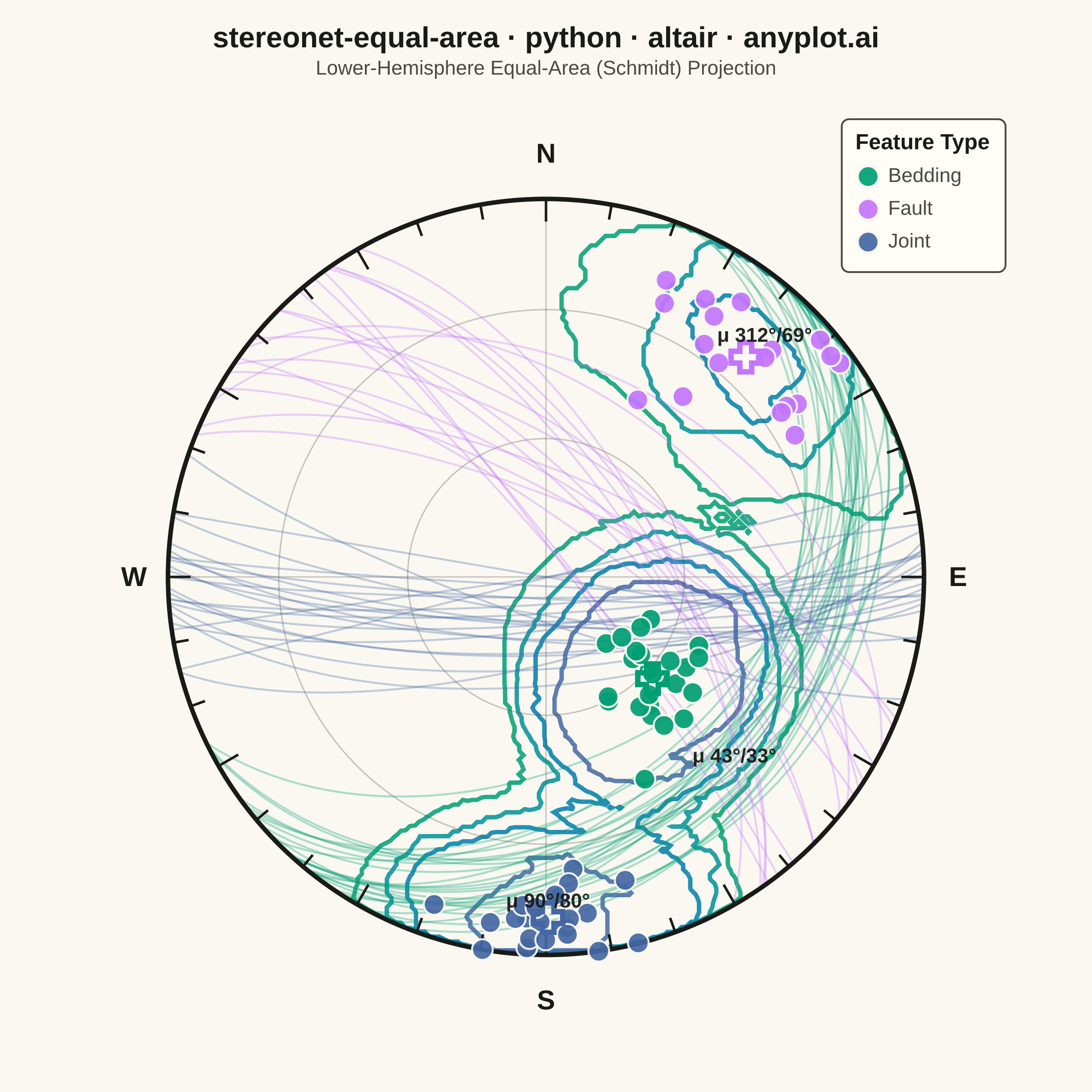
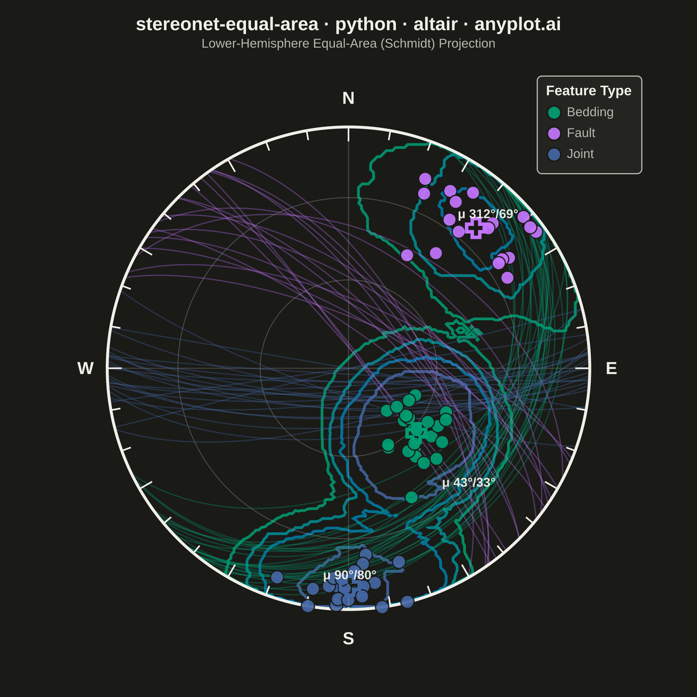
A Schmidt equal-area (lower-hemisphere) stereographic projection for plotting geological structural data. Great circles represent planar features (bedding, faults, joints) by their strike and dip, while poles to planes are plotted as points showing the orientation of the normal to each plane. Density contours highlight preferred orientations in clustered data. This is the standard projection used in structural geology for analyzing fabric elements and kinematic indicators.
""" anyplot.ai
stereonet-equal-area: Structural Geology Stereonet (Equal-Area Projection)
Library: altair 6.2.1 | Python 3.13.13
Quality: 90/100 | Updated: 2026-06-16
"""

import os

import altair as alt
import numpy as np
import pandas as pd
from contourpy import contour_generator


# Theme-adaptive chrome
THEME = os.getenv("ANYPLOT_THEME", "light")
PAGE_BG = "#FAF8F1" if THEME == "light" else "#1A1A17"
ELEVATED_BG = "#FFFDF6" if THEME == "light" else "#242420"
INK = "#1A1A17" if THEME == "light" else "#F0EFE8"
INK_SOFT = "#4A4A44" if THEME == "light" else "#B8B7B0"

# Imprint palette — categorical, theme-independent, hybrid-v3 sort order.
# Geological feature types are abstract categories → canonical order 1→3.
IMPRINT = ["#009E73", "#C475FD", "#4467A3"]
FEATURES = ["Bedding", "Fault", "Joint"]
color_map = dict(zip(FEATURES, IMPRINT, strict=True))
color_scale = alt.Scale(domain=FEATURES, range=IMPRINT)
# Continuous density → imprint_seq (single-polarity, brand green → blue).
IMPRINT_SEQ = ["#009E73", "#4467A3"]

# Data — field measurements of geological structures
np.random.seed(42)

bedding_strike = np.random.normal(45, 12, 25)
bedding_dip = np.random.normal(35, 8, 25)

fault_strike = np.random.normal(310, 15, 18)
fault_dip = np.random.normal(70, 10, 18)

joint_strike = np.random.normal(90, 10, 22)
joint_dip = np.random.normal(80, 7, 22)

strikes = np.concatenate([bedding_strike, fault_strike, joint_strike]) % 360
dips = np.clip(np.concatenate([bedding_dip, fault_dip, joint_dip]), 0, 90)
feature_types = ["Bedding"] * len(bedding_strike) + ["Fault"] * len(fault_strike) + ["Joint"] * len(joint_strike)

# Equal-area (Schmidt) projection: poles to planes
pole_trend = np.radians((strikes + 90) % 360)
pole_r = np.sqrt(2) * np.sin(np.radians(dips) / 2)
pole_x = pole_r * np.sin(pole_trend)
pole_y = pole_r * np.cos(pole_trend)

df_poles = pd.DataFrame(
    {"x": pole_x, "y": pole_y, "feature_type": feature_types, "strike": np.round(strikes, 1), "dip": np.round(dips, 1)}
)

# Great circles for each measurement
gc_rows = []
for i in range(len(strikes)):
    s_rad = np.radians(strikes[i])
    d_rad = np.radians(dips[i])
    dd_rad = s_rad + np.pi / 2
    v1 = np.array([np.sin(s_rad), np.cos(s_rad), 0.0])
    v2 = np.array([np.cos(d_rad) * np.sin(dd_rad), np.cos(d_rad) * np.cos(dd_rad), -np.sin(d_rad)])
    for j, rake in enumerate(np.linspace(0, np.pi, 61)):
        line = np.cos(rake) * v1 + np.sin(rake) * v2
        if line[2] > 0:
            line = -line
        plunge = np.arcsin(-line[2])
        trend = np.arctan2(line[0], line[1])
        r = np.sqrt(2) * np.sin((np.pi / 2 - plunge) / 2)
        gc_rows.append(
            {"x": r * np.sin(trend), "y": r * np.cos(trend), "feature_type": feature_types[i], "gc_id": i, "order": j}
        )
df_gc = pd.DataFrame(gc_rows)

# Primitive circle
r_prim = np.sqrt(2) * np.sin(np.pi / 4)
theta_circ = np.linspace(0, 2 * np.pi, 361)
df_circle = pd.DataFrame({"x": r_prim * np.sin(theta_circ), "y": r_prim * np.cos(theta_circ), "order": range(361)})

# Tick marks every 10 degrees around the perimeter (longer at 30-degree marks)
tick_rows = []
for deg in range(0, 360, 10):
    rad = np.radians(deg)
    tick_len = 0.06 if deg % 30 == 0 else 0.04
    tick_rows.append({"x": r_prim * np.sin(rad), "y": r_prim * np.cos(rad), "tid": deg, "order": 0})
    tick_rows.append(
        {"x": (r_prim - tick_len) * np.sin(rad), "y": (r_prim - tick_len) * np.cos(rad), "tid": deg, "order": 1}
    )
df_ticks = pd.DataFrame(tick_rows)

# Cardinal labels
lbl_r = r_prim + 0.09
df_dirs = pd.DataFrame(
    {"x": [0, lbl_r, 0, -lbl_r], "y": [lbl_r + 0.03, 0, -lbl_r - 0.03, 0], "label": ["N", "E", "S", "W"]}
)

# Equal-area net grid circles at 30 and 60 degree dip
grid_rows = []
for dip_g in [30, 60]:
    r_g = np.sqrt(2) * np.sin(np.radians(dip_g) / 2)
    for j, t in enumerate(np.linspace(0, 2 * np.pi, 181)):
        grid_rows.append({"x": r_g * np.sin(t), "y": r_g * np.cos(t), "level": dip_g, "order": j})
df_grid = pd.DataFrame(grid_rows)

# Grid cross lines (N-S, E-W)
df_cross = pd.DataFrame(
    {
        "x": [0, 0, -r_prim, r_prim],
        "y": [-r_prim, r_prim, 0, 0],
        "line_id": ["NS", "NS", "EW", "EW"],
        "order": [0, 1, 0, 1],
    }
)

# Density field via the Kamb (1959) counting-circle statistic — the standard
# structural-geology method. A counting circle of fixed angular radius is sized
# so that, for a uniform (random) fabric, the expected count within it has a
# standard deviation of `sigma`; the local density is then the number of poles
# falling inside the circle, expressed in units of sigma above that uniform
# expectation. Contours at integer-sigma levels mark statistically significant
# preferred orientations.
n_grid = 160
gx = np.linspace(-r_prim, r_prim, n_grid)
gy = np.linspace(-r_prim, r_prim, n_grid)
gxx, gyy = np.meshgrid(gx, gy)

# Lower-hemisphere 3-D unit vectors for the poles, recovered from their
# equal-area positions (angle from the vertical = 2*arcsin(r/sqrt(2))).
pole_th = 2.0 * np.arcsin(np.clip(pole_r / np.sqrt(2), 0.0, 1.0))
pole_vec = np.column_stack(
    [np.sin(pole_th) * np.sin(pole_trend), np.sin(pole_th) * np.cos(pole_trend), -np.cos(pole_th)]
)

# Grid nodes mapped to the same lower-hemisphere unit vectors.
node_r = np.hypot(gxx, gyy)
node_th = 2.0 * np.arcsin(np.clip(node_r / np.sqrt(2), 0.0, 1.0))
node_tr = np.arctan2(gxx, gyy)
node_vec = np.stack([np.sin(node_th) * np.sin(node_tr), np.sin(node_th) * np.cos(node_tr), -np.cos(node_th)], axis=-1)

# Kamb counting circle: cos-distance threshold and the sigma normalisation.
n_poles = len(pole_vec)
sigma = 3.0
kamb_cos = 1.0 - sigma**2 / (n_poles + sigma**2)
kamb_units = np.sqrt(n_poles * kamb_cos * (1.0 - kamb_cos))

# Count poles inside each node's counting circle (cos of angular distance >=
# threshold), then convert to sigma units with a 0.5 continuity correction.
cos_dist = node_vec @ pole_vec.T
counts = (cos_dist >= kamb_cos).sum(axis=-1)
density = np.clip((counts - 0.5) / kamb_units, 0.0, None)
density[gxx**2 + gyy**2 > r_prim**2] = 0.0

# Smooth, continuous contour polylines via contourpy (the same iso-path engine
# matplotlib uses) — connected vertex chains, not the disconnected per-cell
# segments a marching-squares hand-roll would produce. Contour at integer-sigma
# levels (2σ, 4σ, …); fall back to relative levels for a near-uniform fabric.
dmax = float(np.nanmax(density))
contour_levels = np.arange(2.0, dmax, 2.0)
if len(contour_levels) < 2:
    contour_levels = np.linspace(dmax * 0.3, dmax * 0.9, 4)
cgen = contour_generator(gx, gy, density, line_type="Separate")
contour_rows = []
for li, level in enumerate(contour_levels):
    for si, seg in enumerate(cgen.lines(float(level))):
        for oi, (cx, cy) in enumerate(seg):
            if cx * cx + cy * cy <= r_prim**2 + 1e-9:
                contour_rows.append({"x": cx, "y": cy, "seg_id": f"{li}_{si}", "level": float(li), "order": oi})
df_contours = (
    pd.DataFrame(contour_rows) if contour_rows else pd.DataFrame(columns=["x", "y", "seg_id", "level", "order"])
)

# Mean orientation per feature type; labels pushed radially outward so they
# clear the dense pole clusters they annotate.
mean_rows = []
for ft in FEATURES:
    mask = np.array(feature_types) == ft
    mx, my = float(np.mean(pole_x[mask])), float(np.mean(pole_y[mask]))
    ms, md = float(np.mean(strikes[mask])), float(np.mean(dips[mask]))
    # Offset the label radially off the cluster centroid, but cap its radius so
    # near-perimeter clusters don't push the text onto the cardinal labels.
    norm = np.hypot(mx, my)
    if norm > 1e-6:
        lr = min(norm + 0.30, 0.86)
        lx, ly = mx / norm * lr, my / norm * lr
    else:
        lx, ly = mx, my + 0.30
    mean_rows.append({"x": mx, "y": my, "lx": lx, "ly": ly, "feature_type": ft, "label": f"μ {ms:.0f}°/{md:.0f}°"})
df_means = pd.DataFrame(mean_rows)

# Plot
x_enc = alt.X("x:Q", axis=None, scale=alt.Scale(domain=[-1.3, 1.3]))
y_enc = alt.Y("y:Q", axis=None, scale=alt.Scale(domain=[-1.3, 1.3]))

# Interactive legend selection for highlighting by feature type
selection = alt.selection_point(fields=["feature_type"], bind="legend")

# Density contour lines (imprint_seq, drawn beneath the data)
contour_layer = (
    alt.Chart(df_contours)
    .mark_line(strokeWidth=2.4, strokeCap="round", opacity=0.85)
    .encode(
        x=x_enc,
        y=y_enc,
        detail="seg_id:N",
        order="order:O",
        color=alt.Color(
            "level:Q", scale=alt.Scale(range=IMPRINT_SEQ, domain=[0, len(contour_levels) - 1]), legend=None
        ),
    )
    if len(df_contours) > 0
    else alt.Chart(pd.DataFrame({"x": [0], "y": [0]})).mark_point(size=0).encode(x="x:Q", y="y:Q")
)

grid_circles = (
    alt.Chart(df_grid)
    .mark_line(strokeWidth=0.8, color=INK_SOFT, opacity=0.3)
    .encode(x=x_enc, y=y_enc, detail="level:N", order="order:O")
)

cross_lines = (
    alt.Chart(df_cross)
    .mark_line(strokeWidth=0.8, color=INK_SOFT, opacity=0.3)
    .encode(x=x_enc, y=y_enc, detail="line_id:N", order="order:O")
)

great_circles = (
    alt.Chart(df_gc)
    .mark_line(strokeWidth=1.1)
    .encode(
        x=x_enc,
        y=y_enc,
        detail="gc_id:N",
        order="order:O",
        color=alt.Color("feature_type:N", scale=color_scale, legend=None),
        opacity=alt.condition(selection, alt.value(0.32), alt.value(0.05)),
    )
    .add_params(selection)
)

prim_circle = alt.Chart(df_circle).mark_line(strokeWidth=2.5, color=INK).encode(x=x_enc, y=y_enc, order="order:O")

tick_marks = (
    alt.Chart(df_ticks).mark_line(strokeWidth=1.4, color=INK).encode(x=x_enc, y=y_enc, detail="tid:N", order="order:O")
)

dir_labels = (
    alt.Chart(df_dirs).mark_text(fontSize=15, fontWeight="bold", color=INK).encode(x=x_enc, y=y_enc, text="label:N")
)

poles_layer = (
    alt.Chart(df_poles)
    .mark_point(filled=True, size=130, stroke=PAGE_BG, strokeWidth=1.1)
    .encode(
        x=x_enc,
        y=y_enc,
        color=alt.Color(
            "feature_type:N",
            scale=color_scale,
            title="Feature Type",
            legend=alt.Legend(
                titleFontSize=12,
                labelFontSize=11,
                symbolSize=140,
                orient="top-right",
                titleColor=INK,
                labelColor=INK_SOFT,
                fillColor=ELEVATED_BG,
                strokeColor=INK_SOFT,
                padding=8,
                cornerRadius=4,
            ),
        ),
        opacity=alt.condition(selection, alt.value(0.92), alt.value(0.12)),
        tooltip=[
            alt.Tooltip("feature_type:N", title="Type"),
            alt.Tooltip("strike:Q", title="Strike (°)"),
            alt.Tooltip("dip:Q", title="Dip (°)"),
        ],
    )
    .add_params(selection)
)

# Mean orientation cross markers
mean_markers = (
    alt.Chart(df_means)
    .mark_point(shape="cross", size=260, strokeWidth=3)
    .encode(
        x=x_enc,
        y=y_enc,
        color=alt.Color("feature_type:N", scale=color_scale, legend=None),
        opacity=alt.condition(selection, alt.value(1.0), alt.value(0.12)),
    )
    .add_params(selection)
)

mean_labels = (
    alt.Chart(df_means)
    .mark_text(fontSize=11, fontWeight="bold", color=INK)
    .encode(
        x=alt.X("lx:Q", axis=None, scale=alt.Scale(domain=[-1.3, 1.3])),
        y=alt.Y("ly:Q", axis=None, scale=alt.Scale(domain=[-1.3, 1.3])),
        text="label:N",
        opacity=alt.condition(selection, alt.value(0.95), alt.value(0.1)),
    )
    .add_params(selection)
)

TITLE = "stereonet-equal-area · python · altair · anyplot.ai"
title_fontsize = round(16 * 67 / len(TITLE)) if len(TITLE) > 67 else 16

chart = (
    alt.layer(
        contour_layer,
        grid_circles,
        cross_lines,
        great_circles,
        prim_circle,
        tick_marks,
        dir_labels,
        poles_layer,
        mean_markers,
        mean_labels,
    )
    .properties(
        width=540,
        height=540,
        background=PAGE_BG,
        padding={"left": 6, "right": 6, "top": 6, "bottom": 6},
        title=alt.Title(
            text=TITLE,
            subtitle="Lower-Hemisphere Equal-Area (Schmidt) Projection",
            fontSize=title_fontsize,
            subtitleFontSize=11,
            color=INK,
            subtitleColor=INK_SOFT,
        ),
    )
    .configure_view(fill=PAGE_BG, stroke=None)
)

# Save — square target 2400 × 2400. vl-convert pads outside width/height, so
# pad (never crop) the saved PNG up to the exact canonical canvas.
chart.save(f"plot-{THEME}.png", scale_factor=4.0)
chart.save(f"plot-{THEME}.html")

from PIL import Image


TW, TH = 2400, 2400
_img = Image.open(f"plot-{THEME}.png").convert("RGB")
_w, _h = _img.size
if _w > TW or _h > TH:
    raise SystemExit(
        f"altair vl-convert produced {_w}×{_h}, exceeds target {TW}×{TH}. "
        f"Shrink chart .properties(width=, height=) values and re-render."
    )
if _w < TW or _h < TH:
    _canvas = Image.new("RGB", (TW, TH), PAGE_BG)
    _canvas.paste(_img, ((TW - _w) // 2, (TH - _h) // 2))
    _canvas.save(f"plot-{THEME}.png")
Runnable source as JSON, for any HTTP client: https://api.anyplot.ai/specs/stereonet-equal-area/altair/code. Any spec id and library id listed in llms-full.txt fit the same URL shape; every URL below is complete and callable.
{
  "spec_id": "stereonet-equal-area",
  "language": "python",
  "library": "altair",
  "page": "https://anyplot.ai/stereonet-equal-area/python/altair",
  "hub": "https://anyplot.ai/stereonet-equal-area",
  "code_json": "https://api.anyplot.ai/specs/stereonet-equal-area/altair/code",
  "spec_json": "https://api.anyplot.ai/specs/stereonet-equal-area",
  "render_light_png": "https://storage.googleapis.com/anyplot-images/plots/stereonet-equal-area/python/altair/plot-light.png",
  "render_dark_png": "https://storage.googleapis.com/anyplot-images/plots/stereonet-equal-area/python/altair/plot-dark.png",
  "interactive_light_html": "https://storage.googleapis.com/anyplot-images/plots/stereonet-equal-area/python/altair/plot-light.html",
  "interactive_dark_html": "https://storage.googleapis.com/anyplot-images/plots/stereonet-equal-area/python/altair/plot-dark.html",
  "quality_score": 90.0,
  "license": "MIT",
  "guide": "https://anyplot.ai/llms.txt"
}
Part of Structural Geology Stereonet (Equal-Area Projection) on anyplot.ai.