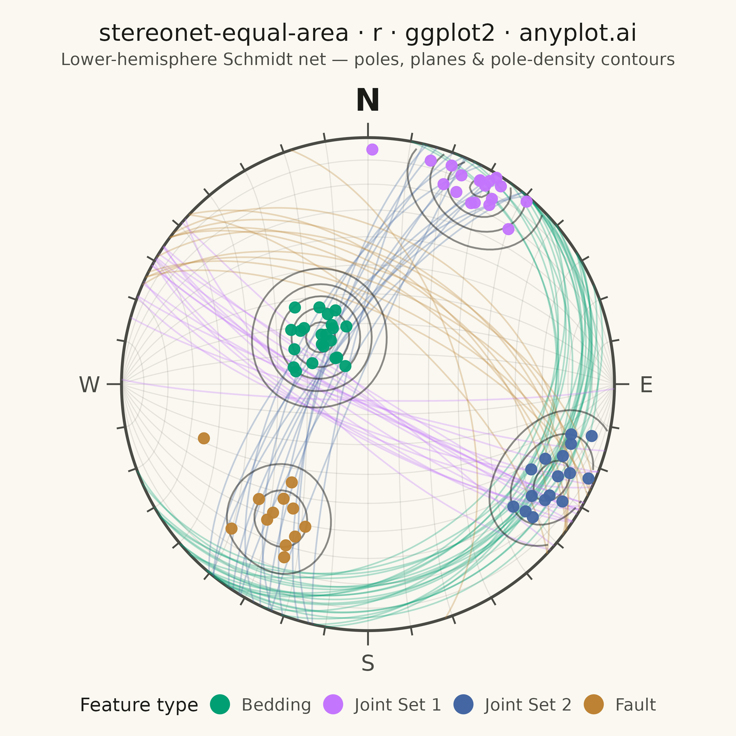
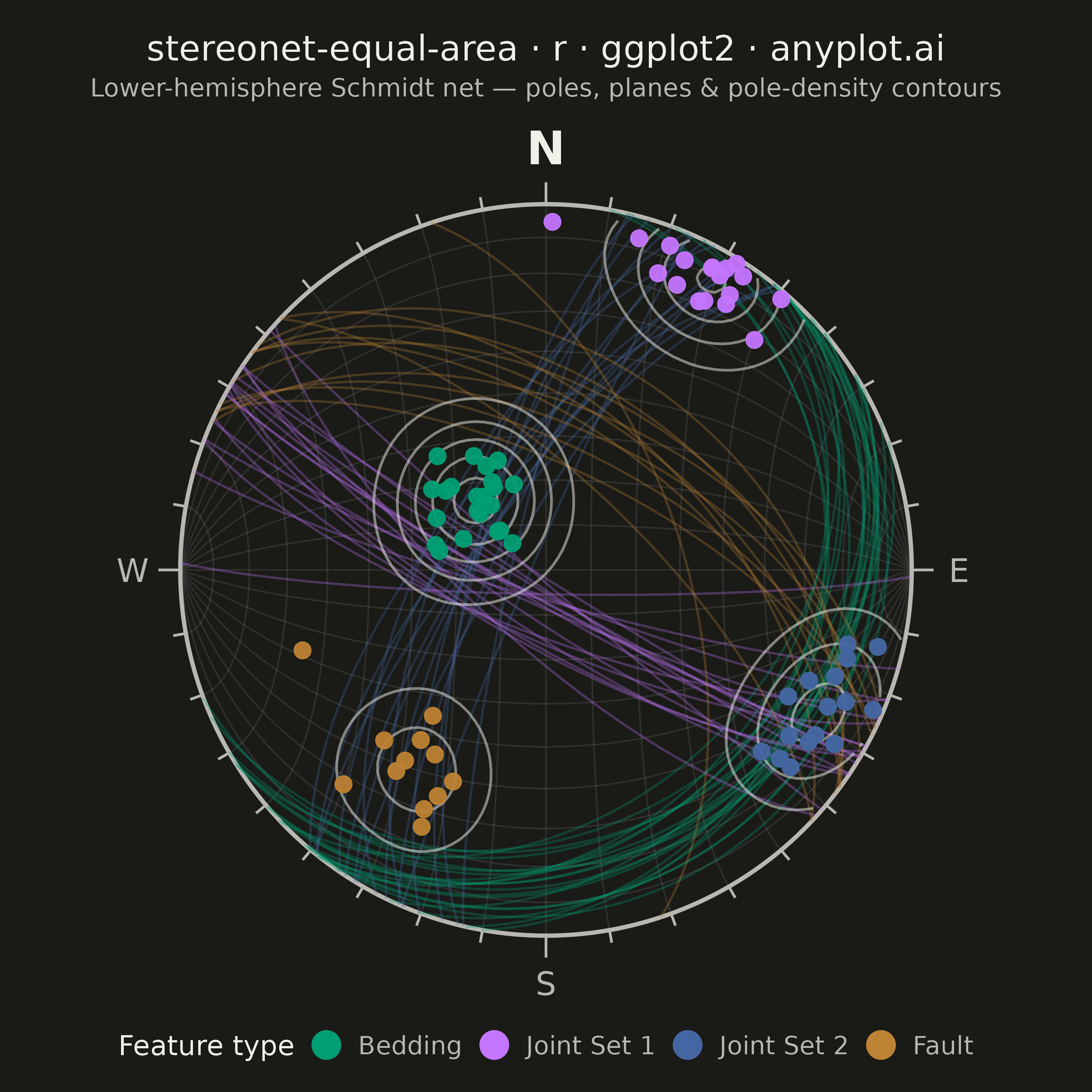
A Schmidt equal-area (lower-hemisphere) stereographic projection for plotting geological structural data. Great circles represent planar features (bedding, faults, joints) by their strike and dip, while poles to planes are plotted as points showing the orientation of the normal to each plane. Density contours highlight preferred orientations in clustered data. This is the standard projection used in structural geology for analyzing fabric elements and kinematic indicators.
#' anyplot.ai
#' stereonet-equal-area: Structural Geology Stereonet (Equal-Area Projection)
#' Library: ggplot2 3.5.1 | R 4.4.1
#' Quality: 91/100 | Created: 2026-06-16

library(ggplot2)
library(dplyr)
library(scales)
library(ragg)

set.seed(42)

# --- Theme tokens -----------------------------------------------------------
THEME       <- Sys.getenv("ANYPLOT_THEME", "light")
PAGE_BG     <- if (THEME == "light") "#FAF8F1" else "#1A1A17"
ELEVATED_BG <- if (THEME == "light") "#FFFDF6" else "#242420"
INK         <- if (THEME == "light") "#1A1A17" else "#F0EFE8"
INK_SOFT    <- if (THEME == "light") "#4A4A44" else "#B8B7B0"
INK_MUTED   <- if (THEME == "light") "#6B6A63" else "#A8A79F"

# Imprint palette — first categorical series is always brand green
IMPRINT_PALETTE <- c("#009E73", "#C475FD", "#4467A3", "#BD8233",
                     "#AE3030", "#2ABCCD", "#954477", "#99B314")

NET_COL  <- alpha(INK, 0.10)   # faint equal-area net grid
PRIM_COL <- INK_SOFT           # primitive circle + ticks
CONT_COL <- alpha(INK, 0.50)   # density contour overlay

# --- Projection helpers (lower-hemisphere Schmidt / equal-area) -------------
# Equal-area radius of a downward line: r = sqrt(1 - sin(plunge)). North is +y,
# East is +x, azimuth measured clockwise from North.
deg2rad <- function(d) d * pi / 180

project_line <- function(trend, plunge) {
  z <- sin(deg2rad(plunge))            # downward direction cosine
  r <- sqrt(pmax(0, 1 - z))            # equal-area radial distance (primitive = 1)
  tr <- deg2rad(trend)
  data.frame(x = r * sin(tr), y = r * cos(tr))
}

# Project a downward unit vector given as (North, East, Down) components.
project_vec <- function(N, E, D) {
  r <- sqrt(pmax(0, 1 - D))
  h <- sqrt(N^2 + E^2)
  s <- ifelse(h > 0, r / h, 0)
  data.frame(x = E * s, y = N * s)
}

# Great circle of a plane (right-hand-rule strike, dip), lower hemisphere.
great_circle <- function(strike, dip, n = 160) {
  S  <- deg2rad(strike)
  Dr <- deg2rad(dip)
  # u = horizontal strike line, d = down-dip line; both unit and orthogonal.
  u <- c(cos(S), sin(S), 0)
  d <- c(-cos(Dr) * sin(S), cos(Dr) * cos(S), sin(Dr))
  phi <- seq(0, pi, length.out = n)   # lower-hemisphere half (Down >= 0)
  N <- cos(phi) * u[1] + sin(phi) * d[1]
  E <- cos(phi) * u[2] + sin(phi) * d[2]
  D <- cos(phi) * u[3] + sin(phi) * d[3]
  project_vec(N, E, D)
}

# --- Equal-area net grid (meridians + small circles about the E-W axis) -----
net_arcs <- list()
gi <- 0
lambda <- seq(0, pi, length.out = 120)
for (g in seq(-80, 80, 10)) {           # meridians: great circles through E & W
  gr <- deg2rad(g)
  N <- sin(lambda) * -sin(gr)
  E <- cos(lambda)
  D <- sin(lambda) * cos(gr)
  gi <- gi + 1
  net_arcs[[gi]] <- transform(project_vec(N, E, D), grp = gi)
}
for (b in seq(10, 170, 10)) {           # small circles: cones about the E-W axis
  br <- deg2rad(b)
  N <- sin(br) * cos(lambda)
  E <- rep(cos(br), length(lambda))
  D <- sin(br) * sin(lambda)
  gi <- gi + 1
  net_arcs[[gi]] <- transform(project_vec(N, E, D), grp = gi)
}
net <- bind_rows(net_arcs)

# --- Primitive circle, perimeter ticks, cardinal labels ---------------------
ct <- seq(0, 2 * pi, length.out = 400)
primitive <- data.frame(x = cos(ct), y = sin(ct))

ang   <- seq(0, 350, 10)
major <- ang %% 90 == 0
ticks <- data.frame(
  x0 = sin(deg2rad(ang)),
  y0 = cos(deg2rad(ang)),
  x1 = sin(deg2rad(ang)) * ifelse(major, 1.06, 1.035),
  y1 = cos(deg2rad(ang)) * ifelse(major, 1.06, 1.035)
)

cardinal <- data.frame(
  lab = c("E", "S", "W"),
  ang = c(90, 180, 270)
)
cardinal$x <- sin(deg2rad(cardinal$ang)) * 1.13
cardinal$y <- cos(deg2rad(cardinal$ang)) * 1.13

# --- Structural data: bedding, two joint sets, a fault set ------------------
make_set <- function(n, strike_mu, strike_sd, dip_mu, dip_sd, label) {
  data.frame(
    strike       = rnorm(n, strike_mu, strike_sd) %% 360,
    dip          = pmin(89, pmax(2, rnorm(n, dip_mu, dip_sd))),
    feature_type = label
  )
}

measurements <- bind_rows(
  make_set(22, 42,  12, 24, 6, "Bedding"),
  make_set(18, 118, 9,  80, 6, "Joint Set 1"),
  make_set(16, 205, 10, 74, 7, "Joint Set 2"),
  make_set(12, 312, 11, 58, 8, "Fault")
)
feature_levels <- c("Bedding", "Joint Set 1", "Joint Set 2", "Fault")
measurements$feature_type <- factor(measurements$feature_type, levels = feature_levels)

# Poles to planes: plunge 90 - dip toward (strike - 90)
poles <- measurements
pole_xy <- project_line((poles$strike + 270) %% 360, 90 - poles$dip)
poles$x <- pole_xy$x
poles$y <- pole_xy$y

# Great circles for every plane (coloured by feature type)
planes_list <- vector("list", nrow(measurements))
for (i in seq_len(nrow(measurements))) {
  arc <- great_circle(measurements$strike[i], measurements$dip[i])
  arc$grp <- i
  arc$feature_type <- measurements$feature_type[i]
  planes_list[[i]] <- arc
}
planes <- bind_rows(planes_list)

# --- Density field over the projected poles (Kamb-style clustering) ---------
gx <- seq(-1, 1, length.out = 90)
grid <- expand.grid(x = gx, y = gx)
band <- 0.13
dens <- numeric(nrow(grid))
for (i in seq_len(nrow(poles))) {
  dens <- dens + exp(-((grid$x - poles$x[i])^2 + (grid$y - poles$y[i])^2) / (2 * band^2))
}
grid$z <- dens
grid$z[sqrt(grid$x^2 + grid$y^2) > 1] <- NA   # clip to the primitive circle

# --- Plot -------------------------------------------------------------------
p <- ggplot() +
  geom_path(data = net, aes(x, y, group = grp),
            color = NET_COL, linewidth = 0.3) +
  geom_path(data = primitive, aes(x, y),
            color = PRIM_COL, linewidth = 0.8) +
  geom_segment(data = ticks, aes(x = x0, y = y0, xend = x1, yend = y1),
               color = PRIM_COL, linewidth = 0.5) +
  geom_path(data = planes, aes(x, y, group = grp, color = feature_type),
            linewidth = 0.45, alpha = 0.30) +
  geom_contour(data = grid, aes(x, y, z = z),
               color = CONT_COL, linewidth = 0.5, bins = 6) +
  geom_point(data = poles, aes(x, y, color = feature_type),
             size = 2.8, alpha = 0.95, stroke = 0.4) +
  annotate("text", x = 0, y = 1.155, label = "N",
           color = INK, fontface = "bold", size = 6.5) +
  geom_text(data = cardinal, aes(x, y, label = lab),
            color = INK_SOFT, size = 4.6) +
  scale_color_manual(values = IMPRINT_PALETTE[1:4], name = "Feature type") +
  coord_fixed(xlim = c(-1.2, 1.2), ylim = c(-1.2, 1.24),
              expand = FALSE, clip = "off") +
  labs(
    title    = "stereonet-equal-area · r · ggplot2 · anyplot.ai",
    subtitle = "Lower-hemisphere Schmidt net — poles, planes & pole-density contours"
  ) +
  guides(color = guide_legend(override.aes = list(linewidth = 0, size = 5, alpha = 1))) +
  theme_void(base_size = 8) +
  theme(
    plot.background  = element_rect(fill = PAGE_BG, color = PAGE_BG),
    panel.background = element_rect(fill = PAGE_BG, color = NA),
    plot.title       = element_text(color = INK, size = 14, hjust = 0.5,
                                    margin = margin(b = 4)),
    plot.subtitle    = element_text(color = INK_SOFT, size = 10, hjust = 0.5,
                                    margin = margin(b = 6)),
    legend.position  = "bottom",
    legend.title     = element_text(color = INK, size = 11),
    legend.text      = element_text(color = INK_SOFT, size = 10),
    legend.key       = element_rect(fill = PAGE_BG, color = NA),
    plot.margin      = margin(14, 14, 10, 14)
  )

# --- Save -------------------------------------------------------------------
ggsave(
  filename = sprintf("plot-%s.png", THEME),
  plot     = p,
  device   = ragg::agg_png,
  width    = 6,
  height   = 6,
  units    = "in",
  dpi      = 400
)
Runnable source as JSON, for any HTTP client: https://api.anyplot.ai/specs/stereonet-equal-area/ggplot2/code. Any spec id and library id listed in llms-full.txt fit the same URL shape; every URL below is complete and callable.
{
  "spec_id": "stereonet-equal-area",
  "language": "r",
  "library": "ggplot2",
  "page": "https://anyplot.ai/stereonet-equal-area/r/ggplot2",
  "hub": "https://anyplot.ai/stereonet-equal-area",
  "code_json": "https://api.anyplot.ai/specs/stereonet-equal-area/ggplot2/code",
  "spec_json": "https://api.anyplot.ai/specs/stereonet-equal-area",
  "render_light_png": "https://storage.googleapis.com/anyplot-images/plots/stereonet-equal-area/r/ggplot2/plot-light.png",
  "render_dark_png": "https://storage.googleapis.com/anyplot-images/plots/stereonet-equal-area/r/ggplot2/plot-dark.png",
  "quality_score": 91.0,
  "license": "MIT",
  "guide": "https://anyplot.ai/llms.txt"
}
Part of Structural Geology Stereonet (Equal-Area Projection) on anyplot.ai.