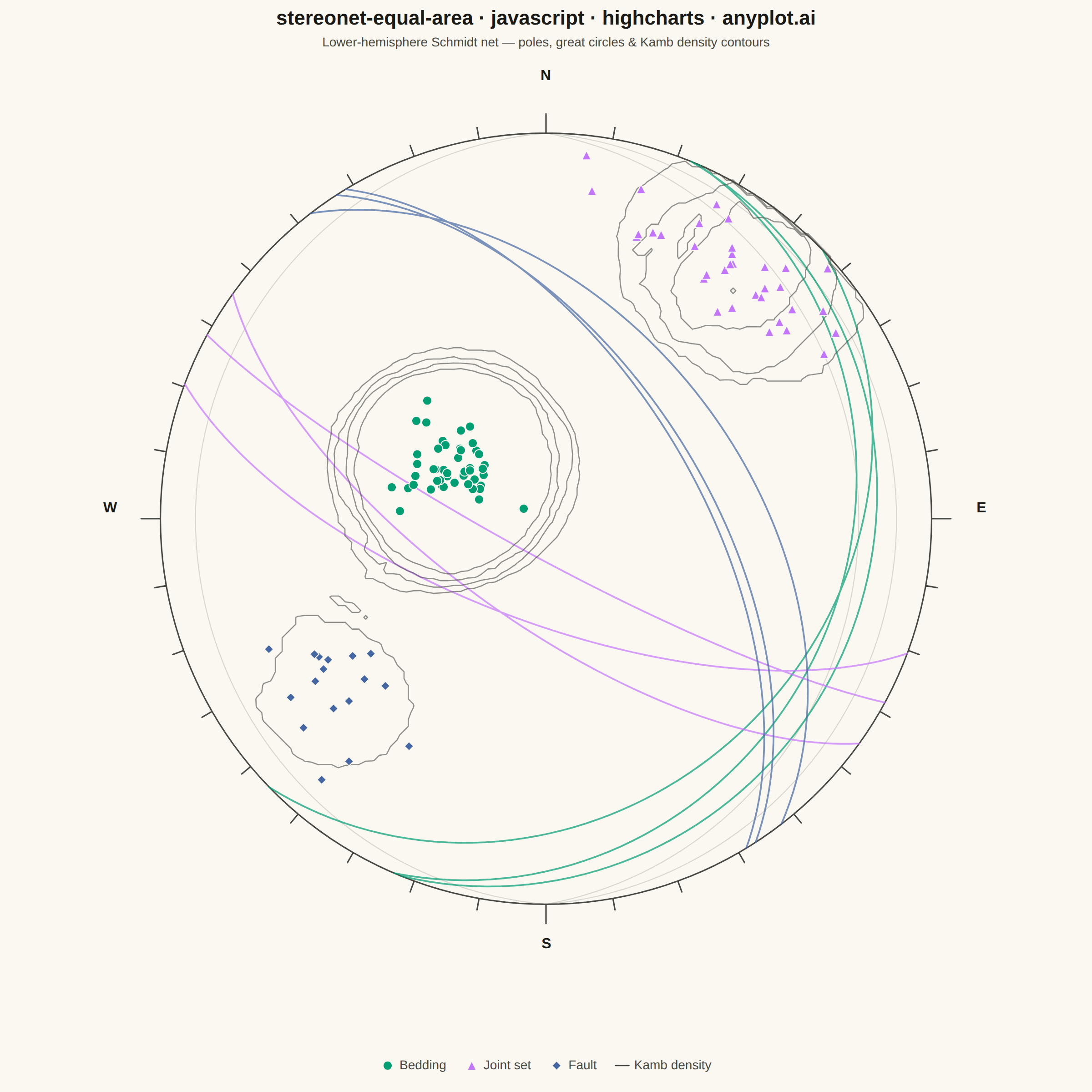
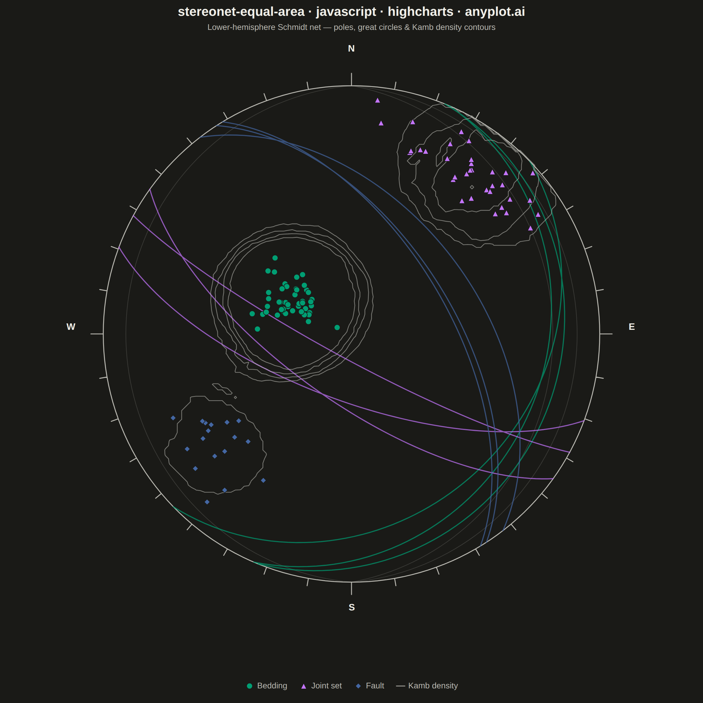
A Schmidt equal-area (lower-hemisphere) stereographic projection for plotting geological structural data. Great circles represent planar features (bedding, faults, joints) by their strike and dip, while poles to planes are plotted as points showing the orientation of the normal to each plane. Density contours highlight preferred orientations in clustered data. This is the standard projection used in structural geology for analyzing fabric elements and kinematic indicators.
// anyplot.ai
// stereonet-equal-area: Structural Geology Stereonet (Equal-Area Projection)
// Library: highcharts 12.6.0 | JavaScript 22.22.3
// Quality: 88/100 | Created: 2026-06-16
//# anyplot-orientation: square
// anyplot.ai
// stereonet-equal-area: Structural Geology Stereonet (Equal-Area Projection)
// Library: Highcharts 12.6.0 | Node 22
// License: Highcharts — commercial license, free for non-commercial use (highcharts.com/license)
// Quality: pending | Created: 2026-06-16

const t = window.ANYPLOT_TOKENS;
const DEG = Math.PI / 180;
const R = 1.0; // primitive (perimeter) radius in axis units

// --- Deterministic RNG (fixed-seed LCG + Box–Muller) -----------------------
let _seed = 20260616;
function rand() {
  _seed = (_seed * 1103515245 + 12345) & 0x7fffffff;
  return _seed / 0x7fffffff;
}
function gauss(mean, sd) {
  let u = 0,
    v = 0;
  while (u === 0) u = rand();
  while (v === 0) v = rand();
  return mean + sd * Math.sqrt(-2 * Math.log(u)) * Math.cos(2 * Math.PI * v);
}

// --- Equal-area (Schmidt, lower-hemisphere) projection ----------------------
// A line of given trend/plunge maps to a planar point. North = +y (top),
// East = +x (right); azimuth measured clockwise from North.
function projLine(trendDeg, plungeDeg) {
  const tr = trendDeg * DEG;
  const rho = (90 - plungeDeg) * DEG; // angular distance from net centre
  const r = R * Math.SQRT2 * Math.sin(rho / 2);
  return [r * Math.sin(tr), r * Math.cos(tr)];
}
// Project a downward direction vector (E, N, U) with U <= 0.
function projVec(e, n, u) {
  const h = Math.hypot(e, n);
  const rho = Math.acos(Math.max(-1, Math.min(1, -u))); // angle from nadir
  const r = R * Math.SQRT2 * Math.sin(rho / 2);
  if (h < 1e-9) return [0, 0];
  return [(r * e) / h, (r * n) / h];
}
// Pole to a plane: normal plunges (90 - dip), trend = dipDir + 180.
function poleXY(dipDir, dip) {
  return projLine(dipDir + 180, 90 - dip);
}
// Great circle of a plane: sweep in-plane lines from one strike end to the other.
function greatCircle(dipDir, dip, steps) {
  const a = dipDir * DEG,
    d = dip * DEG;
  const sx = Math.sin(a - Math.PI / 2),
    sy = Math.cos(a - Math.PI / 2); // strike line (horizontal)
  const tx = Math.cos(d) * Math.sin(a),
    ty = Math.cos(d) * Math.cos(a),
    tz = -Math.sin(d); // dip vector
  const pts = [];
  for (let i = 0; i <= steps; i++) {
    const b = (Math.PI * i) / steps;
    const cb = Math.cos(b),
      sb = Math.sin(b);
    pts.push(projVec(cb * sx + sb * tx, cb * sy + sb * ty, sb * tz));
  }
  return pts;
}

// --- Field data: bedding, joint set, fault (deterministic) ------------------
const features = [
  { name: "Bedding", color: t.palette[0], symbol: "circle", count: 46, ddMean: 118, ddSd: 11, dipMean: 24, dipSd: 6, nGreat: 7 },
  { name: "Joint set", color: t.palette[1], symbol: "triangle", count: 34, ddMean: 212, ddSd: 14, dipMean: 74, dipSd: 8, nGreat: 8 },
  { name: "Fault", color: t.palette[2], symbol: "diamond", count: 17, ddMean: 47, ddSd: 12, dipMean: 60, dipSd: 11, nGreat: 8 },
];

const clamp = (x, lo, hi) => Math.max(lo, Math.min(hi, x));

// Generate every measurement first; collect all poles for the density pass.
const allPoles = [];
features.forEach((f) => {
  f.planes = [];
  for (let i = 0; i < f.count; i++) {
    const dipDir = (gauss(f.ddMean, f.ddSd) + 360) % 360;
    const dip = clamp(gauss(f.dipMean, f.dipSd), 2, 88);
    f.planes.push({ dipDir, dip });
    allPoles.push(poleXY(dipDir, dip));
  }
});

// --- Kamb density contours over the pole population -------------------------
// Kamb (1959): count poles falling inside a counting circle whose area is sized
// so the expected uniform count is 3σ. Contours are drawn at successive σ levels
// above that uniform background via marching squares over an equal-area grid.
function kambContours(poles) {
  const n = poles.length;
  const rc = Math.sqrt(9 / (n + 9)); // counting-circle radius (3σ), primitive R=1
  const rc2 = rc * rc;
  const E = n * rc2; // expected count under a uniform distribution
  const sigma = Math.sqrt(E * (1 - rc2));
  const NX = 120,
    NY = 120,
    span = 2.1,
    x0 = -1.05,
    y0 = -1.05;
  const dx = span / (NX - 1),
    dy = span / (NY - 1);
  const grid = new Float64Array(NX * NY);
  let maxC = 0;
  for (let j = 0; j < NY; j++) {
    const gy = y0 + j * dy;
    for (let i = 0; i < NX; i++) {
      const gx = x0 + i * dx;
      if (gx * gx + gy * gy > 1.0) continue; // only count inside the primitive
      let c = 0;
      for (const p of poles) {
        const ex = p[0] - gx,
          ey = p[1] - gy;
        if (ex * ex + ey * ey <= rc2) c++;
      }
      grid[j * NX + i] = c;
      if (c > maxC) maxC = c;
    }
  }
  // Contour levels in σ above the uniform background; keep those the data reaches.
  let levels = [2, 4, 6, 8].map((k) => E + k * sigma).filter((l) => l < maxC);
  if (levels.length === 0) levels = [0.5 * maxC];

  const frac = (a, b, level) => (level - a) / (b - a);
  function edgePt(e, v0, v1, v2, v3, level, xL, yB) {
    if (e === 0) return [xL + dx * frac(v0, v1, level), yB]; // bottom: BL→BR
    if (e === 1) return [xL + dx, yB + dy * frac(v1, v2, level)]; // right: BR→TR
    if (e === 2) return [xL + dx * frac(v3, v2, level), yB + dy]; // top: TL→TR
    return [xL, yB + dy * frac(v0, v3, level)]; // left: BL→TL
  }
  // Marching-squares segment table (edges 0=bottom 1=right 2=top 3=left).
  const tbl = {
    1: [[3, 0]], 2: [[0, 1]], 3: [[3, 1]], 4: [[1, 2]],
    5: [[3, 0], [1, 2]], 6: [[0, 2]], 7: [[3, 2]], 8: [[2, 3]],
    9: [[0, 2]], 10: [[0, 1], [2, 3]], 11: [[1, 2]], 12: [[3, 1]],
    13: [[0, 1]], 14: [[3, 0]],
  };
  const data = [];
  for (const level of levels) {
    for (let j = 0; j < NY - 1; j++) {
      for (let i = 0; i < NX - 1; i++) {
        const v0 = grid[j * NX + i],
          v1 = grid[j * NX + i + 1],
          v2 = grid[(j + 1) * NX + i + 1],
          v3 = grid[(j + 1) * NX + i];
        let idx = 0;
        if (v0 > level) idx |= 1;
        if (v1 > level) idx |= 2;
        if (v2 > level) idx |= 4;
        if (v3 > level) idx |= 8;
        const segs = tbl[idx];
        if (!segs) continue;
        const xL = x0 + i * dx,
          yB = y0 + j * dy;
        for (const [a, b] of segs) {
          data.push(edgePt(a, v0, v1, v2, v3, level, xL, yB));
          data.push(edgePt(b, v0, v1, v2, v3, level, xL, yB));
          data.push([null, null]);
        }
      }
    }
  }
  return data;
}
const contourData = kambContours(allPoles);

// --- Subtle equal-area net graticule (10° spacing about the N–S axis) -------
const netData = [];
function pushPath(pts) {
  for (const p of pts) netData.push(p);
  netData.push([null, null]);
}
// Meridians: planes striking N–S, dipping E/W — they pass through N and S.
for (let dip = 10; dip <= 80; dip += 10) {
  pushPath(greatCircle(90, dip, 90));
  pushPath(greatCircle(270, dip, 90));
}
pushPath(greatCircle(90, 90, 90)); // straight N–S diameter
pushPath(greatCircle(0, 90, 90)); // straight E–W diameter
// Small circles: cones about the horizontal N–S axis (latitude lines).
for (let colat = 10; colat <= 170; colat += 10) {
  if (colat === 90) continue; // coincides with the E–W diameter
  const k = colat * DEG;
  const arc = [];
  for (let j = 0; j <= 90; j++) {
    const phi = Math.PI + (Math.PI * j) / 90; // lower hemisphere (U <= 0)
    arc.push(projVec(Math.sin(k) * Math.cos(phi), Math.cos(k), Math.sin(k) * Math.sin(phi)));
  }
  pushPath(arc);
}

// --- Primitive circle + 10° perimeter tick marks ---------------------------
const frameData = [];
for (let deg = 0; deg <= 360; deg += 2) {
  frameData.push([R * Math.sin(deg * DEG), R * Math.cos(deg * DEG)]);
}
frameData.push([null, null]);
for (let deg = 0; deg < 360; deg += 10) {
  const outer = deg % 90 === 0 ? 1.05 : 1.03;
  frameData.push([R * Math.sin(deg * DEG), R * Math.cos(deg * DEG)]);
  frameData.push([outer * Math.sin(deg * DEG), outer * Math.cos(deg * DEG)]);
  frameData.push([null, null]);
}

// --- Build per-feature pole (scatter) + great-circle (line) series ----------
const series = [];

// Net graticule and frame sit beneath the data.
series.push({
  type: "line",
  name: "Net grid",
  data: netData,
  color: t.grid,
  lineWidth: 1.1,
  enableMouseTracking: false,
  showInLegend: false,
  marker: { enabled: false },
  zIndex: 0,
});
series.push({
  type: "line",
  name: "Primitive",
  data: frameData,
  color: t.inkSoft,
  lineWidth: 1.6,
  enableMouseTracking: false,
  showInLegend: false,
  marker: { enabled: false },
  zIndex: 1,
});

features.forEach((f, idx) => {
  // Poles (scatter) — every measurement; clustering reveals preferred orientation.
  const poleId = "poles-" + idx;
  series.push({
    type: "scatter",
    id: poleId,
    name: f.name,
    data: f.planes.map((p) => poleXY(p.dipDir, p.dip)),
    color: f.color,
    marker: {
      symbol: f.symbol,
      radius: 5,
      lineWidth: 1,
      lineColor: t.pageBg,
    },
    zIndex: 5,
  });

  // Great circles (line) — an evenly sampled subset keeps the net legible.
  const gcData = [];
  const stride = Math.max(1, Math.floor(f.count / f.nGreat));
  for (let i = 0; i < f.count; i += stride) {
    for (const pt of greatCircle(f.planes[i].dipDir, f.planes[i].dip, 80)) gcData.push(pt);
    gcData.push([null, null]);
  }
  series.push({
    type: "line",
    linkedTo: poleId,
    name: f.name + " planes",
    data: gcData,
    color: f.color,
    lineWidth: 1.9,
    opacity: 0.7,
    enableMouseTracking: false,
    marker: { enabled: false },
    zIndex: 3,
  });
});

// Kamb density contours — nested isolines over the pole clusters (zIndex below
// the poles, above the graticule) directly mark preferred orientations.
series.push({
  type: "line",
  name: "Kamb density",
  data: contourData,
  color: t.inkSoft,
  opacity: 0.6,
  lineWidth: 1.3,
  cropThreshold: Infinity, // unsorted marching-squares segments must not be cropped
  enableMouseTracking: false,
  marker: { enabled: false },
  zIndex: 4, // above the graticule & great circles, beneath the pole markers
});

// --- Cardinal labels (N/E/S/W) just outside the primitive ------------------
series.push({
  type: "scatter",
  name: "Cardinals",
  showInLegend: false,
  enableMouseTracking: false,
  color: t.ink,
  marker: { enabled: false },
  dataLabels: {
    enabled: true,
    allowOverlap: true,
    style: { color: t.ink, fontSize: "16px", fontWeight: "600", textOutline: "none" },
  },
  data: [
    { x: 0, y: 1.12, dataLabels: { format: "N" } },
    { x: 1.13, y: 0, dataLabels: { format: "E" } },
    { x: 0, y: -1.13, dataLabels: { format: "S" } },
    { x: -1.13, y: 0, dataLabels: { format: "W" } },
  ],
  zIndex: 6,
});

// --- Chart ------------------------------------------------------------------
Highcharts.chart("container", {
  chart: {
    type: "scatter",
    backgroundColor: "transparent",
    animation: false,
    style: { fontFamily: "inherit" },
    // Symmetric margins make the plot box square (1000×1000) so the net is round.
    marginTop: 70,
    marginBottom: 130,
    marginLeft: 100,
    marginRight: 100,
  },
  credits: { enabled: false },
  colors: t.palette,
  title: {
    text: "stereonet-equal-area · javascript · highcharts · anyplot.ai",
    style: { color: t.ink, fontSize: "22px", fontWeight: "600" },
  },
  subtitle: {
    text: "Lower-hemisphere Schmidt net — poles, great circles & Kamb density contours",
    style: { color: t.inkSoft, fontSize: "14px" },
  },
  xAxis: {
    min: -1.18,
    max: 1.18,
    visible: false,
    startOnTick: false,
    endOnTick: false,
  },
  yAxis: {
    min: -1.18,
    max: 1.18,
    visible: false,
    startOnTick: false,
    endOnTick: false,
    gridLineWidth: 0,
  },
  legend: {
    align: "center",
    verticalAlign: "bottom",
    itemStyle: { color: t.inkSoft, fontSize: "14px" },
    itemHoverStyle: { color: t.ink },
    symbolRadius: 6,
  },
  plotOptions: {
    series: { animation: false, states: { inactive: { opacity: 1 } } },
    scatter: { stickyTracking: false },
  },
  series,
});
Runnable source as JSON, for any HTTP client: https://api.anyplot.ai/specs/stereonet-equal-area/highcharts/code. Any spec id and library id listed in llms-full.txt fit the same URL shape; every URL below is complete and callable.
{
  "spec_id": "stereonet-equal-area",
  "language": "javascript",
  "library": "highcharts",
  "page": "https://anyplot.ai/stereonet-equal-area/javascript/highcharts",
  "hub": "https://anyplot.ai/stereonet-equal-area",
  "code_json": "https://api.anyplot.ai/specs/stereonet-equal-area/highcharts/code",
  "spec_json": "https://api.anyplot.ai/specs/stereonet-equal-area",
  "render_light_png": "https://storage.googleapis.com/anyplot-images/plots/stereonet-equal-area/javascript/highcharts/plot-light.png",
  "render_dark_png": "https://storage.googleapis.com/anyplot-images/plots/stereonet-equal-area/javascript/highcharts/plot-dark.png",
  "interactive_light_html": "https://storage.googleapis.com/anyplot-images/plots/stereonet-equal-area/javascript/highcharts/plot-light.html",
  "interactive_dark_html": "https://storage.googleapis.com/anyplot-images/plots/stereonet-equal-area/javascript/highcharts/plot-dark.html",
  "quality_score": 88.0,
  "license": "MIT",
  "guide": "https://anyplot.ai/llms.txt"
}
Part of Structural Geology Stereonet (Equal-Area Projection) on anyplot.ai.