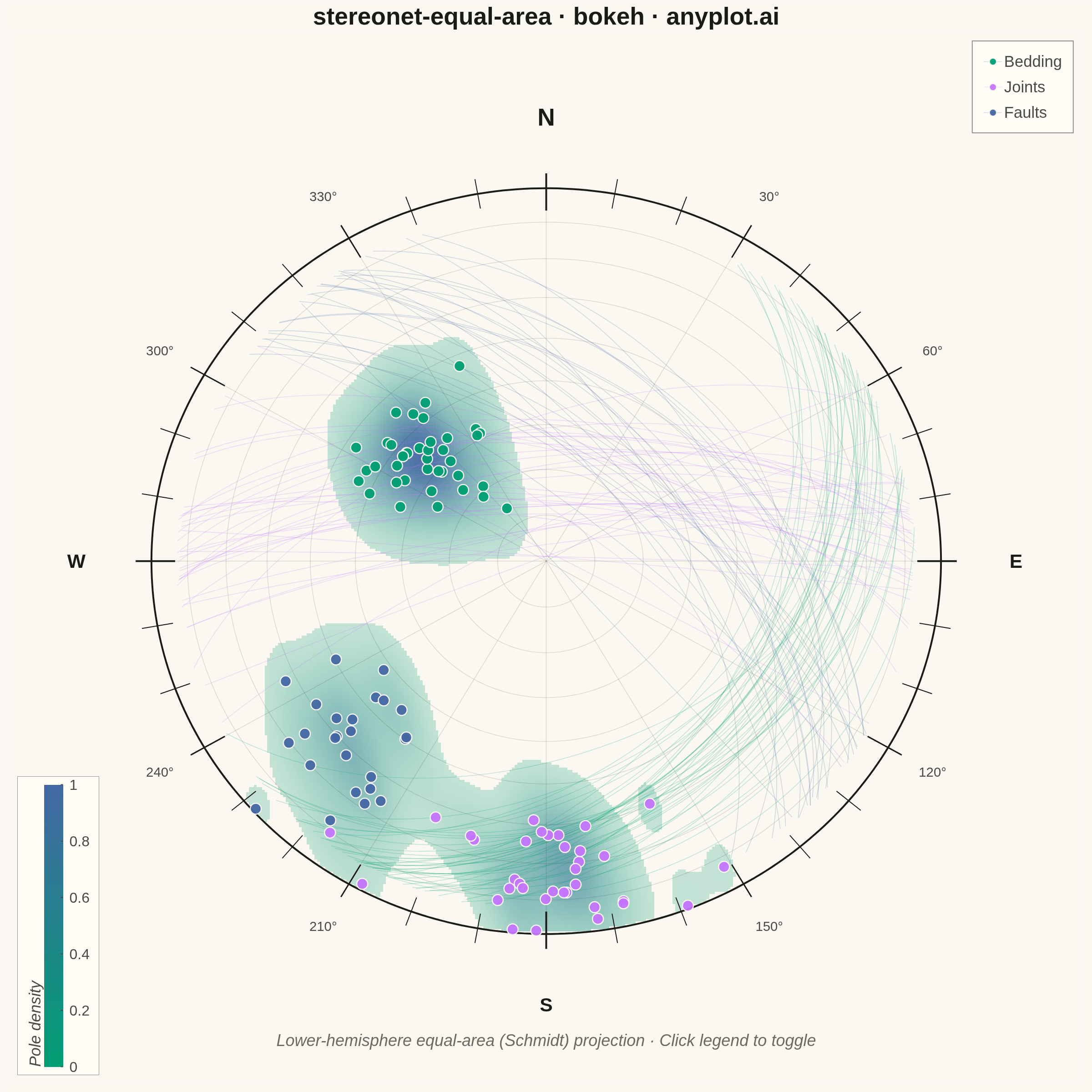
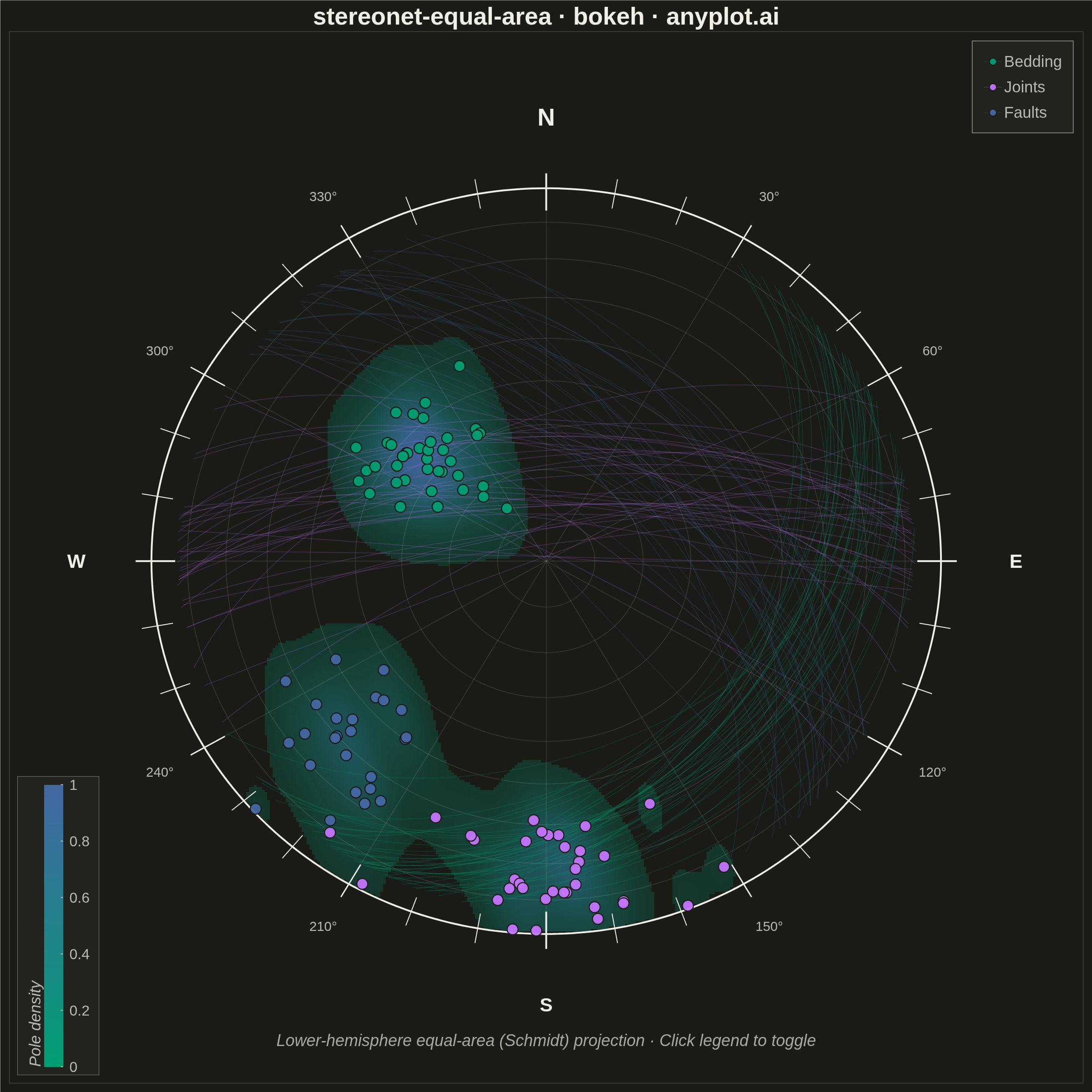
A Schmidt equal-area (lower-hemisphere) stereographic projection for plotting geological structural data. Great circles represent planar features (bedding, faults, joints) by their strike and dip, while poles to planes are plotted as points showing the orientation of the normal to each plane. Density contours highlight preferred orientations in clustered data. This is the standard projection used in structural geology for analyzing fabric elements and kinematic indicators.
""" anyplot.ai
stereonet-equal-area: Structural Geology Stereonet (Equal-Area Projection)
Library: bokeh 3.9.1 | Python 3.13.13
Quality: 90/100 | Updated: 2026-06-16
"""

import os
import sys


# Prevent self-import: this file is named bokeh.py, which shadows the installed
# bokeh package when its directory sits at the front of sys.path.
_this_dir = os.path.dirname(os.path.abspath(__file__))
sys.path = [p for p in sys.path if os.path.abspath(p or ".") != _this_dir]

import time
from pathlib import Path

import numpy as np
from bokeh.io import output_file, save
from bokeh.models import ColorBar, ColumnDataSource, HoverTool, Label, Legend, LegendItem, LinearColorMapper
from bokeh.plotting import figure
from scipy.ndimage import gaussian_filter
from scipy.stats import gaussian_kde
from selenium import webdriver
from selenium.webdriver.chrome.options import Options


# Theme-adaptive chrome
THEME = os.getenv("ANYPLOT_THEME", "light")
PAGE_BG = "#FAF8F1" if THEME == "light" else "#1A1A17"
ELEVATED_BG = "#FFFDF6" if THEME == "light" else "#242420"
INK = "#1A1A17" if THEME == "light" else "#F0EFE8"
INK_SOFT = "#4A4A44" if THEME == "light" else "#B8B7B0"
INK_MUTED = "#6B6A63" if THEME == "light" else "#A8A79F"

# Imprint categorical palette — Bedding/Joints/Faults are abstract geological
# categories, so canonical order: green, lavender, blue.
IMPRINT_PALETTE = ["#009E73", "#C475FD", "#4467A3", "#BD8233", "#AE3030", "#2ABCCD", "#954477", "#99B314"]
colors_map = {"Bedding": IMPRINT_PALETTE[0], "Joints": IMPRINT_PALETTE[1], "Faults": IMPRINT_PALETTE[2]}

# Data - Synthetic structural geology measurements (strike, dip, feature_type)
np.random.seed(42)

# Bedding planes: consistent NE strike with moderate dip
bedding_strike = np.random.normal(45, 12, 40) % 360
bedding_dip = np.random.normal(35, 8, 40).clip(5, 85)

# Joint set: roughly E-W strike, steep dip
joints_strike = np.random.normal(270, 15, 35) % 360
joints_dip = np.random.normal(75, 10, 35).clip(5, 89)

# Fault set: NW strike, moderate-steep dip
faults_strike = np.random.normal(315, 10, 25) % 360
faults_dip = np.random.normal(60, 12, 25).clip(5, 89)

all_strikes = np.concatenate([bedding_strike, joints_strike, faults_strike])
all_dips = np.concatenate([bedding_dip, joints_dip, faults_dip])
all_types = ["Bedding"] * 40 + ["Joints"] * 35 + ["Faults"] * 25

# Equal-area projection: convert pole (plunge, trend) to x, y
R_net = 1.0

pole_trends = (all_strikes + 90 + 180) % 360
pole_plunges = 90.0 - all_dips
pole_trends_rad = np.radians(pole_trends)
pole_plunges_rad = np.radians(pole_plunges)

pole_r = R_net * np.sqrt(2) * np.sin((np.pi / 2 - pole_plunges_rad) / 2)
pole_x = pole_r * np.sin(pole_trends_rad)
pole_y = pole_r * np.cos(pole_trends_rad)

# Great circles for each plane
gc_xs = []
gc_ys = []
gc_types = []

for i in range(len(all_strikes)):
    strike_rad = np.radians(all_strikes[i])
    dip_rad = np.radians(all_dips[i])
    dd_rad = strike_rad + np.pi / 2

    sx = np.sin(strike_rad)
    sy = np.cos(strike_rad)

    dx = np.sin(dd_rad) * np.cos(dip_rad)
    dy = np.cos(dd_rad) * np.cos(dip_rad)
    dz = -np.sin(dip_rad)

    alpha = np.linspace(0, np.pi, 90)
    vx = np.cos(alpha) * sx + np.sin(alpha) * dx
    vy = np.cos(alpha) * sy + np.sin(alpha) * dy
    vz = np.sin(alpha) * dz

    horiz = np.sqrt(vx**2 + vy**2)
    plunge = np.arctan2(-vz, horiz)
    trend = np.arctan2(vx, vy)

    r = R_net * np.sqrt(2) * np.sin((np.pi / 2 - plunge) / 2)
    gx = r * np.sin(trend)
    gy = r * np.cos(trend)

    # Clip great circle points near the primitive circle to reduce edge clutter
    gc_dist = np.sqrt(gx**2 + gy**2)
    keep = gc_dist <= 0.94 * R_net
    gc_xs.append(gx[keep].tolist())
    gc_ys.append(gy[keep].tolist())
    gc_types.append(all_types[i])

# Density grid for pole data using KDE
grid_n = 300
gx_lin = np.linspace(-R_net, R_net, grid_n)
gy_lin = np.linspace(-R_net, R_net, grid_n)
gx_grid, gy_grid = np.meshgrid(gx_lin, gy_lin)

dist_grid = np.sqrt(gx_grid**2 + gy_grid**2)
mask = dist_grid <= R_net

pole_xy = np.vstack([pole_x, pole_y])
kde = gaussian_kde(pole_xy, bw_method=0.2)
density = kde(np.vstack([gx_grid.ravel(), gy_grid.ravel()])).reshape(grid_n, grid_n)
density = gaussian_filter(density, sigma=3)

# Normalize density inside the primitive circle
density_masked = density.copy()
density_masked[~mask] = np.nan
d_min = np.nanmin(density_masked[mask])
d_max = np.nanmax(density_masked[mask])
d_norm = (density_masked - d_min) / (d_max - d_min)

# Continuous data → Imprint sequential cmap (imprint_seq: brand green → blue).
SEQ_LO = (0x00, 0x9E, 0x73)  # #009E73 brand green
SEQ_HI = (0x44, 0x67, 0xA3)  # #4467A3 blue
imprint_seq256 = [
    "#{:02X}{:02X}{:02X}".format(
        int(round(SEQ_LO[0] + (SEQ_HI[0] - SEQ_LO[0]) * t / 255.0)),
        int(round(SEQ_LO[1] + (SEQ_HI[1] - SEQ_LO[1]) * t / 255.0)),
        int(round(SEQ_LO[2] + (SEQ_HI[2] - SEQ_LO[2]) * t / 255.0)),
    )
    for t in range(256)
]

# Build uint32 RGBA density overlay from imprint_seq (vectorized)
img = np.zeros((grid_n, grid_n), dtype=np.uint32)
view = img.view(dtype=np.uint8).reshape((grid_n, grid_n, 4))
visible = mask & (d_norm > 0.06)
v = np.clip(np.where(visible, d_norm, 0.0), 0.0, 1.0)
view[visible, 0] = (SEQ_LO[0] + (SEQ_HI[0] - SEQ_LO[0]) * v[visible]).astype(np.uint8)
view[visible, 1] = (SEQ_LO[1] + (SEQ_HI[1] - SEQ_LO[1]) * v[visible]).astype(np.uint8)
view[visible, 2] = (SEQ_LO[2] + (SEQ_HI[2] - SEQ_LO[2]) * v[visible]).astype(np.uint8)
view[visible, 3] = (45 + 195 * v[visible]).astype(np.uint8)  # alpha rises with density

# Plot - Square format for circular stereonet (2400 x 2400)
p = figure(
    width=2400,
    height=2400,
    title="stereonet-equal-area · bokeh · anyplot.ai",
    x_range=(-1.36, 1.36),
    y_range=(-1.40, 1.42),
    tools="pan,wheel_zoom,reset,save",
    toolbar_location=None,
    match_aspect=True,
    min_border=20,
)

# Density heatmap as Bokeh image_rgba (distinctive Bokeh raster overlay)
p.image_rgba(image=[img], x=-R_net, y=-R_net, dw=2 * R_net, dh=2 * R_net, level="image")

# Density colorbar (imprint_seq) — inset into the empty bottom-left corner so it
# sits with the circular plot rather than floating off to the side.
color_mapper = LinearColorMapper(palette=imprint_seq256, low=0.0, high=1.0)
color_bar = ColorBar(
    color_mapper=color_mapper,
    location="bottom_left",
    orientation="vertical",
    title="Pole density",
    title_text_font_size="26pt",
    title_text_font_style="italic",
    title_text_color=INK_SOFT,
    major_label_text_font_size="24pt",
    major_label_text_color=INK_SOFT,
    label_standoff=14,
    width=42,
    height=620,
    padding=18,
    margin=18,
    background_fill_color=ELEVATED_BG,
    background_fill_alpha=0.85,
    border_line_color=INK_SOFT,
    border_line_alpha=0.6,
    major_tick_line_color=INK_SOFT,
    major_tick_line_width=2,
)
p.add_layout(color_bar)

# Equal-area net grid lines (small circles at 10° dip intervals) — subtle
for dip_angle in range(10, 90, 10):
    dip_rad = np.radians(dip_angle)
    grid_r = R_net * np.sqrt(2) * np.sin(dip_rad / 2)
    theta = np.linspace(0, 2 * np.pi, 180)
    gx = grid_r * np.cos(theta)
    gy = grid_r * np.sin(theta)
    p.line(gx, gy, line_color=INK, line_width=1.5, line_alpha=0.14)

# Great circle grid lines at every 30° azimuth — subtle
for az_deg in range(0, 180, 30):
    az_rad = np.radians(az_deg)
    alpha = np.linspace(0, np.pi, 90)
    vx = np.cos(alpha) * np.sin(az_rad)
    vy = np.cos(alpha) * np.cos(az_rad)
    vz = -np.sin(alpha)
    horiz = np.sqrt(vx**2 + vy**2)
    plunge = np.arctan2(-vz, horiz)
    trend = np.arctan2(vx, vy)
    r = R_net * np.sqrt(2) * np.sin((np.pi / 2 - plunge) / 2)
    grid_gx = r * np.sin(trend)
    grid_gy = r * np.cos(trend)
    p.line(grid_gx, grid_gy, line_color=INK, line_width=1.5, line_alpha=0.14)

# Primitive circle (outer boundary)
theta_circle = np.linspace(0, 2 * np.pi, 360)
circle_x = R_net * np.cos(theta_circle)
circle_y = R_net * np.sin(theta_circle)
p.line(circle_x, circle_y, line_color=INK, line_width=4)

# Tick marks every 10 degrees around perimeter
for deg in range(0, 360, 10):
    rad = np.radians(deg)
    tick_len = 0.06 if deg % 30 == 0 else 0.04
    x_inner = (1.0 - tick_len) * R_net * np.sin(rad)
    y_inner = (1.0 - tick_len) * R_net * np.cos(rad)
    x_outer = 1.04 * R_net * np.sin(rad)
    y_outer = 1.04 * R_net * np.cos(rad)
    lw = 4 if deg % 90 == 0 else (3 if deg % 30 == 0 else 2)
    p.line([x_inner, x_outer], [y_inner, y_outer], line_color=INK, line_width=lw)

# Degree labels every 30 degrees (skip cardinals — labelled separately)
for deg in range(0, 360, 30):
    if deg % 90 == 0:
        continue
    rad = np.radians(deg)
    lx = 1.13 * R_net * np.sin(rad)
    ly = 1.13 * R_net * np.cos(rad)
    p.add_layout(
        Label(
            x=lx,
            y=ly,
            text=f"{deg}°",
            text_font_size="22pt",
            text_align="center",
            text_baseline="middle",
            text_color=INK_SOFT,
        )
    )

# Cardinal direction labels
for deg, label in [(0, "N"), (90, "E"), (180, "S"), (270, "W")]:
    rad = np.radians(deg)
    lx = 1.19 * R_net * np.sin(rad)
    ly = 1.19 * R_net * np.cos(rad)
    fs = "40pt" if label == "N" else "32pt"
    p.add_layout(
        Label(
            x=lx,
            y=ly,
            text=label,
            text_font_size=fs,
            text_font_style="bold",
            text_align="center",
            text_baseline="middle",
            text_color=INK,
        )
    )

# Great circles by feature type
renderers_gc = {}
for ftype in ["Bedding", "Joints", "Faults"]:
    idxs = [j for j, t in enumerate(gc_types) if t == ftype]
    fxs = [gc_xs[j] for j in idxs]
    fys = [gc_ys[j] for j in idxs]
    r = p.multi_line(fxs, fys, line_color=colors_map[ftype], line_width=1.6, line_alpha=0.22)
    renderers_gc[ftype] = r

# Poles by feature type with HoverTool
renderers_pole = {}
for ftype in ["Bedding", "Joints", "Faults"]:
    idxs = [j for j, t in enumerate(all_types) if t == ftype]
    px = pole_x[idxs]
    py = pole_y[idxs]
    strikes = all_strikes[idxs]
    dips = all_dips[idxs]
    source = ColumnDataSource(
        data={"x": px, "y": py, "strike": np.round(strikes, 1), "dip": np.round(dips, 1), "type": [ftype] * len(idxs)}
    )
    r = p.scatter(
        "x", "y", source=source, size=24, color=colors_map[ftype], line_color=PAGE_BG, line_width=2.5, alpha=0.95
    )
    renderers_pole[ftype] = r

# HoverTool for pole data (Bokeh distinctive feature)
hover = HoverTool(
    renderers=list(renderers_pole.values()),
    tooltips=[("Type", "@type"), ("Strike", "@strike°"), ("Dip", "@dip°")],
    point_policy="snap_to_data",
)
p.add_tools(hover)

# Interactive legend (click to hide/show — Bokeh distinctive feature)
legend_items = []
for ftype in ["Bedding", "Joints", "Faults"]:
    legend_items.append(LegendItem(label=ftype, renderers=[renderers_gc[ftype], renderers_pole[ftype]]))

legend = Legend(items=legend_items, location="top_right")
legend.label_text_font_size = "26pt"
legend.label_text_color = INK_SOFT
legend.glyph_height = 40
legend.glyph_width = 40
legend.spacing = 16
legend.background_fill_color = ELEVATED_BG
legend.background_fill_alpha = 0.92
legend.border_line_color = INK_SOFT
legend.border_line_alpha = 0.6
legend.border_line_width = 2
legend.padding = 24
legend.margin = 20
legend.click_policy = "hide"
p.add_layout(legend)

# Style
p.title.text_font_size = "40pt"
p.title.align = "center"
p.title.text_color = INK
p.xaxis.visible = False
p.yaxis.visible = False
p.xgrid.visible = False
p.ygrid.visible = False
p.outline_line_color = None
p.background_fill_color = PAGE_BG
p.border_fill_color = PAGE_BG

# Subtitle annotation
p.add_layout(
    Label(
        x=0,
        y=-1.31,
        text="Lower-hemisphere equal-area (Schmidt) projection · Click legend to toggle",
        text_font_size="27pt",
        text_align="center",
        text_color=INK_MUTED,
        text_font_style="italic",
    )
)

# Save — interactive HTML + headless-Chrome screenshot (export_png is unreliable here)
output_file(f"plot-{THEME}.html")
save(p)

W, H = 2400, 2400
opts = Options()
for arg in (
    "--headless=new",
    "--no-sandbox",
    "--disable-dev-shm-usage",
    "--disable-gpu",
    f"--window-size={W},{H}",
    "--hide-scrollbars",
):
    opts.add_argument(arg)
driver = webdriver.Chrome(options=opts)
driver.set_window_size(W, H)
driver.get(f"file://{Path(f'plot-{THEME}.html').resolve()}")
time.sleep(2)  # let bokeh's JS render the canvas

# Headless Chrome's viewport is smaller than the requested window (window chrome),
# which shrinks the screenshot below the figure's height. Compensate so the inner
# viewport is exactly W x H, then re-render.
inner_w = driver.execute_script("return window.innerWidth")
inner_h = driver.execute_script("return window.innerHeight")
driver.set_window_size(W + (W - inner_w), H + (H - inner_h))
time.sleep(2)
driver.save_screenshot(f"plot-{THEME}.png")
driver.quit()
Runnable source as JSON, for any HTTP client: https://api.anyplot.ai/specs/stereonet-equal-area/bokeh/code. Any spec id and library id listed in llms-full.txt fit the same URL shape; every URL below is complete and callable.
{
  "spec_id": "stereonet-equal-area",
  "language": "python",
  "library": "bokeh",
  "page": "https://anyplot.ai/stereonet-equal-area/python/bokeh",
  "hub": "https://anyplot.ai/stereonet-equal-area",
  "code_json": "https://api.anyplot.ai/specs/stereonet-equal-area/bokeh/code",
  "spec_json": "https://api.anyplot.ai/specs/stereonet-equal-area",
  "render_light_png": "https://storage.googleapis.com/anyplot-images/plots/stereonet-equal-area/python/bokeh/plot-light.png",
  "render_dark_png": "https://storage.googleapis.com/anyplot-images/plots/stereonet-equal-area/python/bokeh/plot-dark.png",
  "interactive_light_html": "https://storage.googleapis.com/anyplot-images/plots/stereonet-equal-area/python/bokeh/plot-light.html",
  "interactive_dark_html": "https://storage.googleapis.com/anyplot-images/plots/stereonet-equal-area/python/bokeh/plot-dark.html",
  "quality_score": 90.0,
  "license": "MIT",
  "guide": "https://anyplot.ai/llms.txt"
}
Part of Structural Geology Stereonet (Equal-Area Projection) on anyplot.ai.