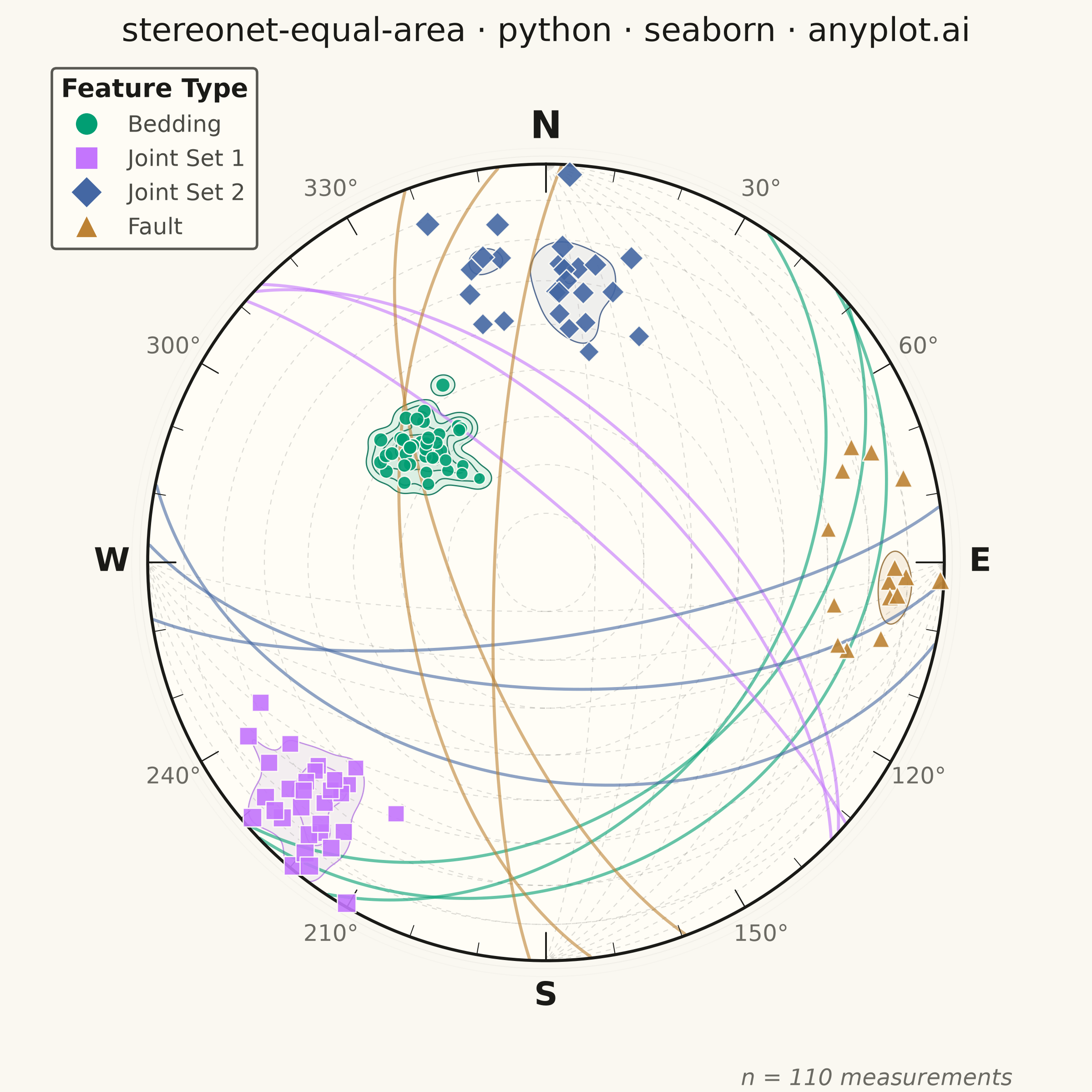
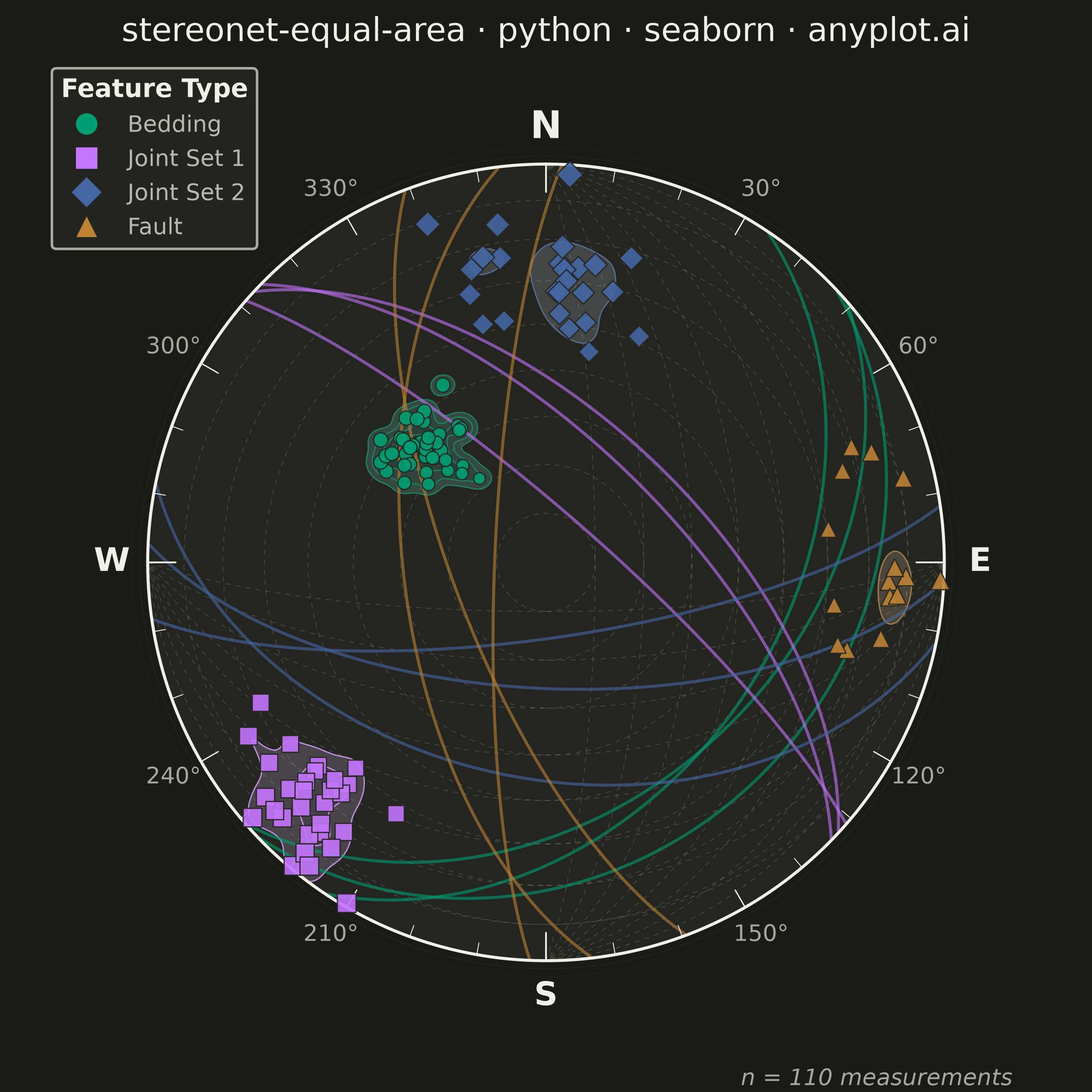
A Schmidt equal-area (lower-hemisphere) stereographic projection for plotting geological structural data. Great circles represent planar features (bedding, faults, joints) by their strike and dip, while poles to planes are plotted as points showing the orientation of the normal to each plane. Density contours highlight preferred orientations in clustered data. This is the standard projection used in structural geology for analyzing fabric elements and kinematic indicators.
""" anyplot.ai
stereonet-equal-area: Structural Geology Stereonet (Equal-Area Projection)
Library: seaborn 0.13.2 | Python 3.13.13
Quality: 93/100 | Updated: 2026-06-16
"""

import os

import matplotlib.pyplot as plt
import numpy as np
import pandas as pd
import seaborn as sns


# Theme-adaptive chrome (Imprint palette)
THEME = os.getenv("ANYPLOT_THEME", "light")
PAGE_BG = "#FAF8F1" if THEME == "light" else "#1A1A17"
ELEVATED_BG = "#FFFDF6" if THEME == "light" else "#242420"
INK = "#1A1A17" if THEME == "light" else "#F0EFE8"
INK_SOFT = "#4A4A44" if THEME == "light" else "#B8B7B0"
INK_MUTED = "#6B6A63" if THEME == "light" else "#A8A79F"

# Data - field measurements from a geological mapping campaign
np.random.seed(42)

bedding_strike = np.random.normal(45, 8, 40) % 360
bedding_dip = np.clip(np.random.normal(35, 5, 40), 1, 89)

joint1_strike = np.random.normal(315, 10, 30) % 360
joint1_dip = np.clip(np.random.normal(75, 8, 30), 1, 89)

joint2_strike = np.random.normal(90, 12, 25) % 360
joint2_dip = np.clip(np.random.normal(60, 10, 25), 1, 89)

fault_strike = np.random.normal(180, 15, 15) % 360
fault_dip = np.clip(np.random.normal(70, 10, 15), 1, 89)

strikes = np.concatenate([bedding_strike, joint1_strike, joint2_strike, fault_strike])
dips = np.concatenate([bedding_dip, joint1_dip, joint2_dip, fault_dip])
feature_types = ["Bedding"] * 40 + ["Joint Set 1"] * 30 + ["Joint Set 2"] * 25 + ["Fault"] * 15

df = pd.DataFrame({"strike": strikes, "dip": dips, "feature_type": feature_types})

# Equal-area projection: convert pole trend/plunge to x, y
pole_trend = (df["strike"].values + 270) % 360
pole_plunge = 90 - df["dip"].values
pole_trend_rad = np.radians(pole_trend)
pole_plunge_rad = np.radians(pole_plunge)
pole_r = np.sqrt(2) * np.sin((np.pi / 2 - pole_plunge_rad) / 2)
df["pole_x"] = pole_r * np.sin(pole_trend_rad)
df["pole_y"] = pole_r * np.cos(pole_trend_rad)

# Scale marker size by dip angle for visual hierarchy (steeper dips = larger markers)
df["marker_size"] = 80 + (df["dip"] / 90) * 120

# Imprint palette, canonical order 1->4 (abstract feature types, no semantic cue)
sns.set_theme(
    style="white",
    rc={"figure.facecolor": PAGE_BG, "axes.facecolor": PAGE_BG, "text.color": INK, "font.family": "DejaVu Sans"},
)
feature_colors = ["#009E73", "#C475FD", "#4467A3", "#BD8233"]
palette = sns.color_palette(feature_colors)
feature_names = ["Bedding", "Joint Set 1", "Joint Set 2", "Fault"]
palette_dict = dict(zip(feature_names, palette, strict=True))

# Square canvas: 6 x 6 in @ dpi=400 -> 2400 x 2400 px (hard contract)
fig, ax = plt.subplots(figsize=(6, 6), dpi=400, facecolor=PAGE_BG)
ax.set_facecolor(PAGE_BG)
ax.set_aspect("equal")

# Subtle outer glow ring for depth
for ring_r, ring_alpha in [(1.02, 0.05), (1.04, 0.025)]:
    glow = plt.Circle((0, 0), ring_r, fill=False, color=INK_SOFT, linewidth=0.4, alpha=ring_alpha)
    ax.add_patch(glow)

# Primitive circle with refined styling (elevated surface lifts the net off the page)
theta_circle = np.linspace(0, 2 * np.pi, 300)
ax.fill(np.sin(theta_circle), np.cos(theta_circle), color=ELEVATED_BG, zorder=0)
ax.plot(np.sin(theta_circle), np.cos(theta_circle), color=INK, linewidth=1.2, zorder=4)

# Grid: small circles (constant plunge)
for plunge_deg in range(10, 90, 10):
    r = np.sqrt(2) * np.sin((np.pi / 2 - np.radians(plunge_deg)) / 2)
    grid_circle = plt.Circle(
        (0, 0), r, fill=False, color=INK, alpha=0.15, linewidth=0.4, linestyle=(0, (5, 5)), zorder=1
    )
    ax.add_patch(grid_circle)

# Grid: great circles for N-S and E-W reference planes
for ref_strike in [0, 90]:
    ref_strike_rad = np.radians(ref_strike)
    for ref_dip in range(10, 90, 10):
        ref_dip_rad = np.radians(ref_dip)
        alpha = np.linspace(0.01, np.pi - 0.01, 150)
        vx = np.cos(alpha) * np.sin(ref_strike_rad) + np.sin(alpha) * np.cos(ref_dip_rad) * np.cos(ref_strike_rad)
        vy = np.cos(alpha) * np.cos(ref_strike_rad) - np.sin(alpha) * np.cos(ref_dip_rad) * np.sin(ref_strike_rad)
        vz = -np.sin(alpha) * np.sin(ref_dip_rad)
        gc_plunge = np.arcsin(np.clip(-vz, -1, 1))
        gc_trend = np.arctan2(vx, vy)
        gc_r = np.sqrt(2) * np.sin((np.pi / 2 - gc_plunge) / 2)
        gc_x = gc_r * np.sin(gc_trend)
        gc_y = gc_r * np.cos(gc_trend)
        ax.plot(gc_x, gc_y, color=INK, alpha=0.15, linewidth=0.4, linestyle=(0, (5, 5)), zorder=1)

# Tick marks every 10 degrees with graduated lengths
for azimuth in range(0, 360, 10):
    az_rad = np.radians(azimuth)
    if azimuth % 90 == 0:
        tick_inner, tick_lw = 0.93, 0.7
    elif azimuth % 30 == 0:
        tick_inner, tick_lw = 0.95, 0.5
    else:
        tick_inner, tick_lw = 0.97, 0.35
    ax.plot(
        [tick_inner * np.sin(az_rad), np.sin(az_rad)],
        [tick_inner * np.cos(az_rad), np.cos(az_rad)],
        color=INK,
        linewidth=tick_lw,
        zorder=4,
    )

# Cardinal direction labels with refined typography
for az, label in [(0, "N"), (90, "E"), (180, "S"), (270, "W")]:
    az_rad = np.radians(az)
    fontsize = 15 if label == "N" else 13
    ax.text(
        1.09 * np.sin(az_rad),
        1.09 * np.cos(az_rad),
        label,
        ha="center",
        va="center",
        fontsize=fontsize,
        fontweight="bold",
        color=INK,
        zorder=6,
    )

# Degree labels every 30 degrees (skip cardinals)
for az in range(30, 360, 30):
    if az in [90, 180, 270]:
        continue
    az_rad = np.radians(az)
    ax.text(
        1.08 * np.sin(az_rad),
        1.08 * np.cos(az_rad),
        f"{az}°",
        ha="center",
        va="center",
        fontsize=9,
        color=INK_MUTED,
        zorder=6,
    )

# Density contours per feature type using seaborn kdeplot with hue
n_collections_before = len(ax.collections)
n_lines_before = len(ax.lines)

sns.kdeplot(
    data=df,
    x="pole_x",
    y="pole_y",
    hue="feature_type",
    hue_order=feature_names,
    palette=[sns.desaturate(c, 0.45) for c in feature_colors],
    fill=True,
    levels=5,
    thresh=0.2,
    alpha=0.22,
    bw_adjust=0.7,
    ax=ax,
    zorder=2,
    legend=False,
)
sns.kdeplot(
    data=df,
    x="pole_x",
    y="pole_y",
    hue="feature_type",
    hue_order=feature_names,
    palette=[sns.desaturate(c, 0.6) for c in feature_colors],
    levels=5,
    thresh=0.2,
    linewidths=0.5,
    bw_adjust=0.7,
    ax=ax,
    zorder=2,
    legend=False,
)

# Clip density contours to the primitive circle
clip_circle = plt.Circle((0, 0), 1.0, transform=ax.transData, fill=False)
ax.add_patch(clip_circle)
clip_circle.set_visible(False)
for c in ax.collections[n_collections_before:]:
    c.set_clip_path(clip_circle)
for line in ax.lines[n_lines_before:]:
    line.set_clip_path(clip_circle)

# Great circles for representative planes (3 per feature type)
for feature_type in df["feature_type"].unique():
    subset = df[df["feature_type"] == feature_type]
    indices = np.linspace(0, len(subset) - 1, min(3, len(subset)), dtype=int)
    for idx in indices:
        row = subset.iloc[idx]
        s_rad = np.radians(row["strike"])
        d_rad = np.radians(row["dip"])
        alpha = np.linspace(0.01, np.pi - 0.01, 200)
        vx = np.cos(alpha) * np.sin(s_rad) + np.sin(alpha) * np.cos(d_rad) * np.cos(s_rad)
        vy = np.cos(alpha) * np.cos(s_rad) - np.sin(alpha) * np.cos(d_rad) * np.sin(s_rad)
        vz = -np.sin(alpha) * np.sin(d_rad)
        gc_plunge = np.arcsin(np.clip(-vz, -1, 1))
        gc_trend = np.arctan2(vx, vy)
        gc_r = np.sqrt(2) * np.sin((np.pi / 2 - gc_plunge) / 2)
        gc_x = gc_r * np.sin(gc_trend)
        gc_y = gc_r * np.cos(gc_trend)
        ax.plot(gc_x, gc_y, color=palette_dict[feature_type], linewidth=1.2, alpha=0.6, zorder=3)

# Poles using seaborn scatterplot with hue, shape and size encoding
marker_map = {"Bedding": "o", "Joint Set 1": "s", "Joint Set 2": "D", "Fault": "^"}
sns.scatterplot(
    data=df,
    x="pole_x",
    y="pole_y",
    hue="feature_type",
    hue_order=feature_names,
    style="feature_type",
    style_order=feature_names,
    markers=marker_map,
    size="marker_size",
    sizes=(22, 55),
    palette=palette_dict,
    edgecolor=ELEVATED_BG,
    linewidth=0.5,
    alpha=0.9,
    ax=ax,
    zorder=5,
    legend=False,
)

# Style
ax.set_xlim(-1.22, 1.22)
ax.set_ylim(-1.22, 1.22)
ax.set_xlabel("")
ax.set_ylabel("")
ax.set_xticks([])
ax.set_yticks([])
sns.despine(ax=ax, left=True, bottom=True)

# Build a custom legend with marker shapes matching the plot
handles = []
for ft in feature_names:
    handles.append(
        plt.Line2D(
            [0],
            [0],
            marker=marker_map[ft],
            color="none",
            markerfacecolor=palette_dict[ft],
            markersize=9,
            markeredgecolor=ELEVATED_BG,
            markeredgewidth=0.5,
            label=ft,
        )
    )

legend = ax.legend(
    handles=handles,
    title="Feature Type",
    loc="upper left",
    fontsize=9,
    title_fontsize=10,
    framealpha=0.92,
    facecolor=ELEVATED_BG,
    edgecolor=INK_SOFT,
    fancybox=True,
    shadow=False,
    bbox_to_anchor=(-0.02, 1.02),
)
legend.get_title().set_fontweight("semibold")
legend.get_title().set_color(INK)
for text in legend.get_texts():
    text.set_color(INK_SOFT)

# Measurement count annotation
n_total = len(df)
ax.text(
    0.98,
    -0.02,
    f"n = {n_total} measurements",
    transform=ax.transAxes,
    fontsize=9,
    color=INK_MUTED,
    ha="right",
    va="top",
    style="italic",
)

ax.set_title(
    "stereonet-equal-area · python · seaborn · anyplot.ai", fontsize=13, fontweight="medium", color=INK, pad=14
)

# Save (no bbox_inches='tight' -> exact 2400 x 2400 px)
fig.subplots_adjust(left=0.04, right=0.96, top=0.93, bottom=0.04)
plt.savefig(f"plot-{THEME}.png", dpi=400, facecolor=PAGE_BG)
Runnable source as JSON, for any HTTP client: https://api.anyplot.ai/specs/stereonet-equal-area/seaborn/code. Any spec id and library id listed in llms-full.txt fit the same URL shape; every URL below is complete and callable.
{
  "spec_id": "stereonet-equal-area",
  "language": "python",
  "library": "seaborn",
  "page": "https://anyplot.ai/stereonet-equal-area/python/seaborn",
  "hub": "https://anyplot.ai/stereonet-equal-area",
  "code_json": "https://api.anyplot.ai/specs/stereonet-equal-area/seaborn/code",
  "spec_json": "https://api.anyplot.ai/specs/stereonet-equal-area",
  "render_light_png": "https://storage.googleapis.com/anyplot-images/plots/stereonet-equal-area/python/seaborn/plot-light.png",
  "render_dark_png": "https://storage.googleapis.com/anyplot-images/plots/stereonet-equal-area/python/seaborn/plot-dark.png",
  "quality_score": 93.0,
  "license": "MIT",
  "guide": "https://anyplot.ai/llms.txt"
}
Part of Structural Geology Stereonet (Equal-Area Projection) on anyplot.ai.