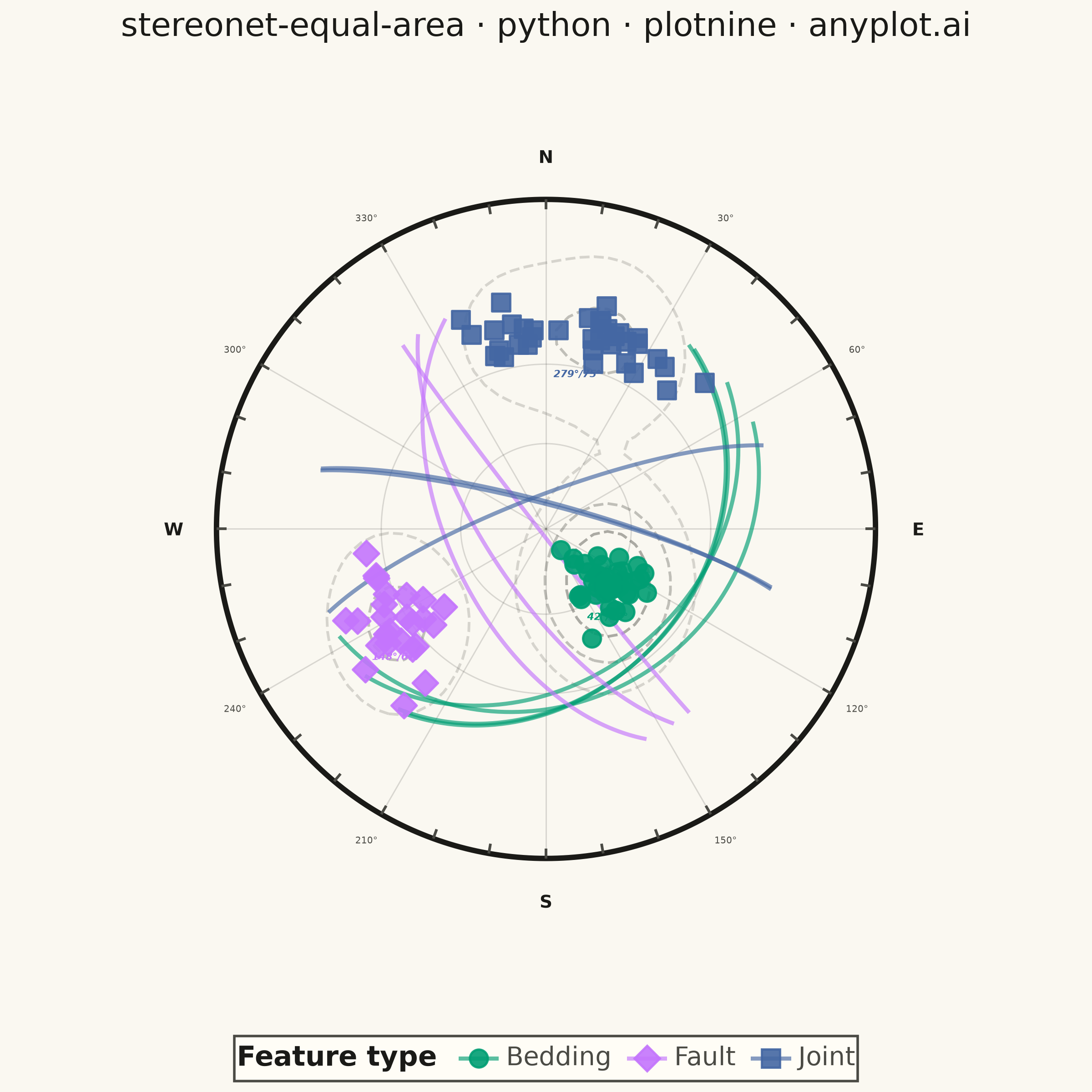
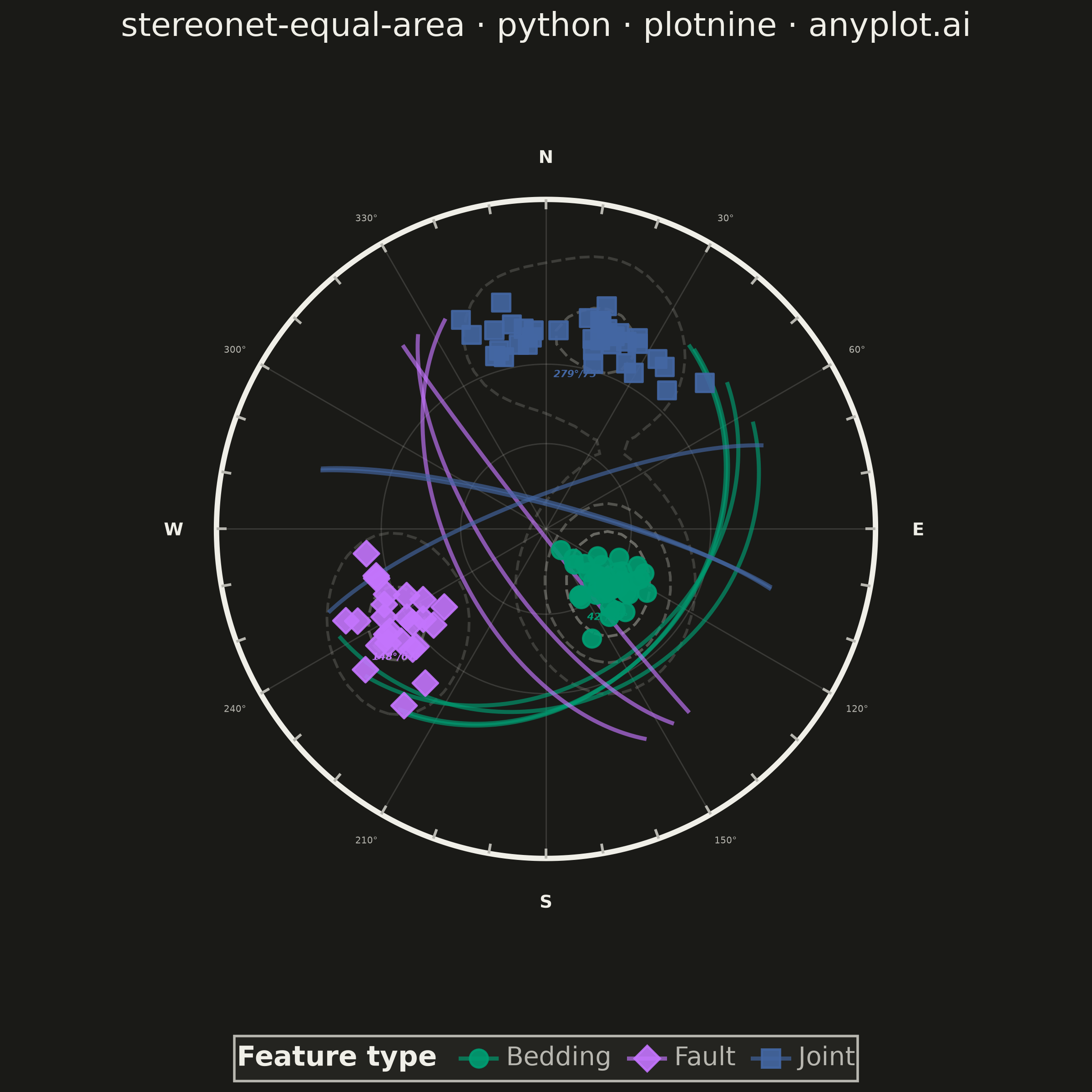
A Schmidt equal-area (lower-hemisphere) stereographic projection for plotting geological structural data. Great circles represent planar features (bedding, faults, joints) by their strike and dip, while poles to planes are plotted as points showing the orientation of the normal to each plane. Density contours highlight preferred orientations in clustered data. This is the standard projection used in structural geology for analyzing fabric elements and kinematic indicators.
""" anyplot.ai
stereonet-equal-area: Structural Geology Stereonet (Equal-Area Projection)
Library: plotnine 0.15.7 | Python 3.13.13
Quality: 90/100 | Updated: 2026-06-16
"""

import os

import numpy as np
import pandas as pd
from plotnine import (
    aes,
    after_stat,
    coord_fixed,
    element_blank,
    element_rect,
    element_text,
    geom_density_2d,
    geom_path,
    geom_point,
    geom_segment,
    geom_text,
    ggplot,
    labs,
    scale_alpha_continuous,
    scale_color_manual,
    scale_shape_manual,
    scale_x_continuous,
    scale_y_continuous,
    theme,
)


# Theme tokens (see prompts/default-style-guide.md "Theme-adaptive Chrome")
THEME = os.getenv("ANYPLOT_THEME", "light")
PAGE_BG = "#FAF8F1" if THEME == "light" else "#1A1A17"
ELEVATED_BG = "#FFFDF6" if THEME == "light" else "#242420"
INK = "#1A1A17" if THEME == "light" else "#F0EFE8"
INK_SOFT = "#4A4A44" if THEME == "light" else "#B8B7B0"
INK_MUTED = "#6B6A63" if THEME == "light" else "#A8A79F"

# Imprint palette — Bedding=brand green (always first), Fault=lavender, Joint=blue
IMPRINT = {"Bedding": "#009E73", "Fault": "#C475FD", "Joint": "#4467A3"}
SHAPES = {"Bedding": "o", "Fault": "D", "Joint": "s"}

# Data — geological field measurements (strike/dip for bedding, faults, joints)
np.random.seed(42)

bedding_strike = np.random.normal(45, 12, 40)
bedding_dip = np.clip(np.random.normal(30, 8, 40), 5, 85)

fault_strike = np.random.normal(150, 15, 25)
fault_dip = np.clip(np.random.normal(65, 10, 25), 10, 88)

joint_strike = np.random.normal(280, 20, 35)
joint_dip = np.clip(np.random.normal(75, 8, 35), 15, 89)

strikes = np.concatenate([bedding_strike, fault_strike, joint_strike]) % 360
dips = np.concatenate([bedding_dip, fault_dip, joint_dip])
feature_types = ["Bedding"] * 40 + ["Fault"] * 25 + ["Joint"] * 35

# Primitive circle radius for the Schmidt equal-area projection
r_prim = np.sqrt(2)

# Compute poles to planes (equal-area lower-hemisphere projection)
pole_trend = np.radians((strikes + 90) % 360)
pole_plunge = np.radians(90 - dips)
pole_r = np.sqrt(2) * np.sin((np.pi / 2 - pole_plunge) / 2)
pole_x = pole_r * np.sin(pole_trend)
pole_y = pole_r * np.cos(pole_trend)
poles_df = pd.DataFrame({"x": pole_x, "y": pole_y, "feature_type": feature_types})

# Compute great circles for a few representative planes per feature type
gc_rows = []
gc_indices = {"Bedding": [0, 10, 20, 30], "Fault": [40, 48, 56], "Joint": [65, 75, 85]}
gc_id = 0
for ftype, indices in gc_indices.items():
    for idx in indices:
        if idx >= len(strikes):
            continue
        strike_rad = np.radians(strikes[idx])
        dip_rad = np.radians(dips[idx])
        strike_vec = np.array([np.sin(strike_rad), np.cos(strike_rad), 0.0])
        dip_dir_rad = strike_rad + np.pi / 2
        dip_vec = np.array(
            [np.sin(dip_dir_rad) * np.cos(dip_rad), np.cos(dip_dir_rad) * np.cos(dip_rad), -np.sin(dip_rad)]
        )
        for a in np.linspace(-np.pi / 2, np.pi / 2, 181):
            pt = np.cos(a) * dip_vec + np.sin(a) * strike_vec
            if pt[2] > 0:
                pt = -pt
            horiz = np.sqrt(pt[0] ** 2 + pt[1] ** 2)
            plunge = np.arctan2(-pt[2], horiz)
            trend = np.arctan2(pt[0], pt[1])
            r = np.sqrt(2) * np.sin((np.pi / 2 - plunge) / 2)
            x, y = r * np.sin(trend), r * np.cos(trend)
            if x**2 + y**2 <= r_prim**2 * 1.01:
                gc_rows.append({"x": x, "y": y, "feature_type": ftype, "gc_id": f"{ftype}_{gc_id}"})
        gc_id += 1

gc_df = pd.DataFrame(gc_rows)

# Stereonet net — primitive circle
circle_angles = np.linspace(0, 2 * np.pi, 361)
prim_df = pd.DataFrame({"x": r_prim * np.cos(circle_angles), "y": r_prim * np.sin(circle_angles)})

# Equal-area net grid — small circles at 30 deg dip intervals
grid_rows = []
for dip_interval in range(30, 90, 30):
    plunge_rad = np.radians(90 - dip_interval)
    r_circle = np.sqrt(2) * np.sin((np.pi / 2 - plunge_rad) / 2)
    for angle in np.linspace(0, 2 * np.pi, 181):
        grid_rows.append(
            {"x": r_circle * np.cos(angle), "y": r_circle * np.sin(angle), "grid_id": f"dip_{dip_interval}"}
        )

# Radial lines at 30 deg azimuth intervals
for az in range(0, 360, 30):
    az_rad = np.radians(az)
    for t in np.linspace(0, r_prim, 50):
        grid_rows.append({"x": t * np.sin(az_rad), "y": t * np.cos(az_rad), "grid_id": f"az_{az}"})

grid_df = pd.DataFrame(grid_rows)

# Degree tick marks every 10 degrees around the perimeter
tick_rows = []
for deg in range(0, 360, 10):
    rad = np.radians(deg)
    inner, outer = r_prim * 0.97, r_prim * 1.0
    tick_rows.append(
        {"x1": inner * np.sin(rad), "y1": inner * np.cos(rad), "x2": outer * np.sin(rad), "y2": outer * np.cos(rad)}
    )
tick_df = pd.DataFrame(tick_rows)

# Cardinal direction labels
dir_labels = []
for deg, label in [(0, "N"), (90, "E"), (180, "S"), (270, "W")]:
    rad = np.radians(deg)
    offset = r_prim * 1.13
    dir_labels.append({"x": offset * np.sin(rad), "y": offset * np.cos(rad), "label": label})
dir_df = pd.DataFrame(dir_labels)

# Degree labels every 30 degrees (excluding cardinal directions)
deg_labels = []
for deg in range(0, 360, 30):
    if deg in (0, 90, 180, 270):
        continue
    rad = np.radians(deg)
    offset = r_prim * 1.09
    deg_labels.append({"x": offset * np.sin(rad), "y": offset * np.cos(rad), "label": f"{deg}°"})
deg_label_df = pd.DataFrame(deg_labels)

# Mean strike/dip annotation per cluster (geological context)
annotations = []
for ftype in ["Bedding", "Fault", "Joint"]:
    mask = poles_df["feature_type"] == ftype
    cx, cy = poles_df.loc[mask, "x"].mean(), poles_df.loc[mask, "y"].mean()
    mean_strike = strikes[np.array(feature_types) == ftype].mean()
    mean_dip = dips[np.array(feature_types) == ftype].mean()
    annotations.append({"x": cx, "y": cy - 0.14, "feature_type": ftype, "label": f"{mean_strike:.0f}°/{mean_dip:.0f}°"})
annot_df = pd.DataFrame(annotations)

# Plot — layered grammar of graphics on the equal-area net
plot = (
    ggplot()
    # Equal-area net grid (subtle, theme-adaptive)
    + geom_path(aes(x="x", y="y", group="grid_id"), data=grid_df, color=INK, size=0.3, alpha=0.15)
    # Primitive circle (projection boundary)
    + geom_path(aes(x="x", y="y"), data=prim_df, color=INK, size=1.2)
    # Perimeter degree ticks
    + geom_segment(aes(x="x1", y="y1", xend="x2", yend="y2"), data=tick_df, color=INK_SOFT, size=0.6)
    # Pole concentration density contours
    + geom_density_2d(
        aes(x="x", y="y", alpha=after_stat("level")),
        data=poles_df,
        color=INK_MUTED,
        size=0.6,
        linetype="dashed",
        show_legend=False,
    )
    + scale_alpha_continuous(range=(0.25, 0.7))
    # Great circles for representative planes
    + geom_path(aes(x="x", y="y", color="feature_type", group="gc_id"), data=gc_df, size=0.9, alpha=0.65)
    # Poles to planes
    + geom_point(
        aes(x="x", y="y", color="feature_type", shape="feature_type"), data=poles_df, size=3.5, alpha=0.9, stroke=0.5
    )
    # Cardinal direction labels
    + geom_text(aes(x="x", y="y", label="label"), data=dir_df, size=7, fontweight="bold", color=INK)
    # Perimeter degree labels
    + geom_text(aes(x="x", y="y", label="label"), data=deg_label_df, size=3.6, color=INK_SOFT)
    # Mean strike/dip per cluster
    + geom_text(
        aes(x="x", y="y", label="label", color="feature_type"),
        data=annot_df,
        size=4.0,
        fontstyle="italic",
        fontweight="bold",
        show_legend=False,
    )
    + scale_color_manual(name="Feature type", values=IMPRINT)
    + scale_shape_manual(name="Feature type", values=SHAPES)
    + coord_fixed(ratio=1)
    + scale_x_continuous(limits=(-1.85, 1.85))
    + scale_y_continuous(limits=(-1.85, 1.85))
    + labs(title="stereonet-equal-area · python · plotnine · anyplot.ai")
    + theme(
        figure_size=(6, 6),
        plot_background=element_rect(fill=PAGE_BG, color=PAGE_BG),
        panel_background=element_rect(fill=PAGE_BG, color=PAGE_BG),
        legend_background=element_rect(fill=ELEVATED_BG, color=INK_SOFT),
        legend_key=element_rect(fill=ELEVATED_BG, color=ELEVATED_BG),
        plot_title=element_text(size=13, ha="center", color=INK),
        legend_title=element_text(size=11, weight="bold", color=INK),
        legend_text=element_text(size=10, color=INK_SOFT),
        legend_position="bottom",
        axis_title=element_blank(),
        axis_text=element_blank(),
        axis_ticks=element_blank(),
        axis_line=element_blank(),
        panel_grid_major=element_blank(),
        panel_grid_minor=element_blank(),
        panel_border=element_blank(),
    )
)

# Save (2400 x 2400 px square at dpi=400)
plot.save(f"plot-{THEME}.png", dpi=400, width=6, height=6, units="in")
Runnable source as JSON, for any HTTP client: https://api.anyplot.ai/specs/stereonet-equal-area/plotnine/code. Any spec id and library id listed in llms-full.txt fit the same URL shape; every URL below is complete and callable.
{
  "spec_id": "stereonet-equal-area",
  "language": "python",
  "library": "plotnine",
  "page": "https://anyplot.ai/stereonet-equal-area/python/plotnine",
  "hub": "https://anyplot.ai/stereonet-equal-area",
  "code_json": "https://api.anyplot.ai/specs/stereonet-equal-area/plotnine/code",
  "spec_json": "https://api.anyplot.ai/specs/stereonet-equal-area",
  "render_light_png": "https://storage.googleapis.com/anyplot-images/plots/stereonet-equal-area/python/plotnine/plot-light.png",
  "render_dark_png": "https://storage.googleapis.com/anyplot-images/plots/stereonet-equal-area/python/plotnine/plot-dark.png",
  "quality_score": 90.0,
  "license": "MIT",
  "guide": "https://anyplot.ai/llms.txt"
}
Part of Structural Geology Stereonet (Equal-Area Projection) on anyplot.ai.