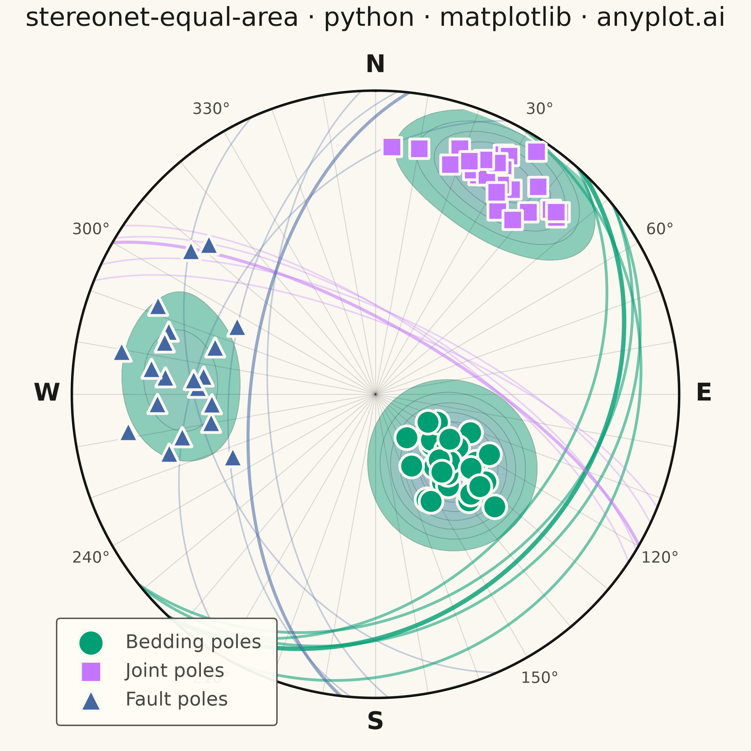
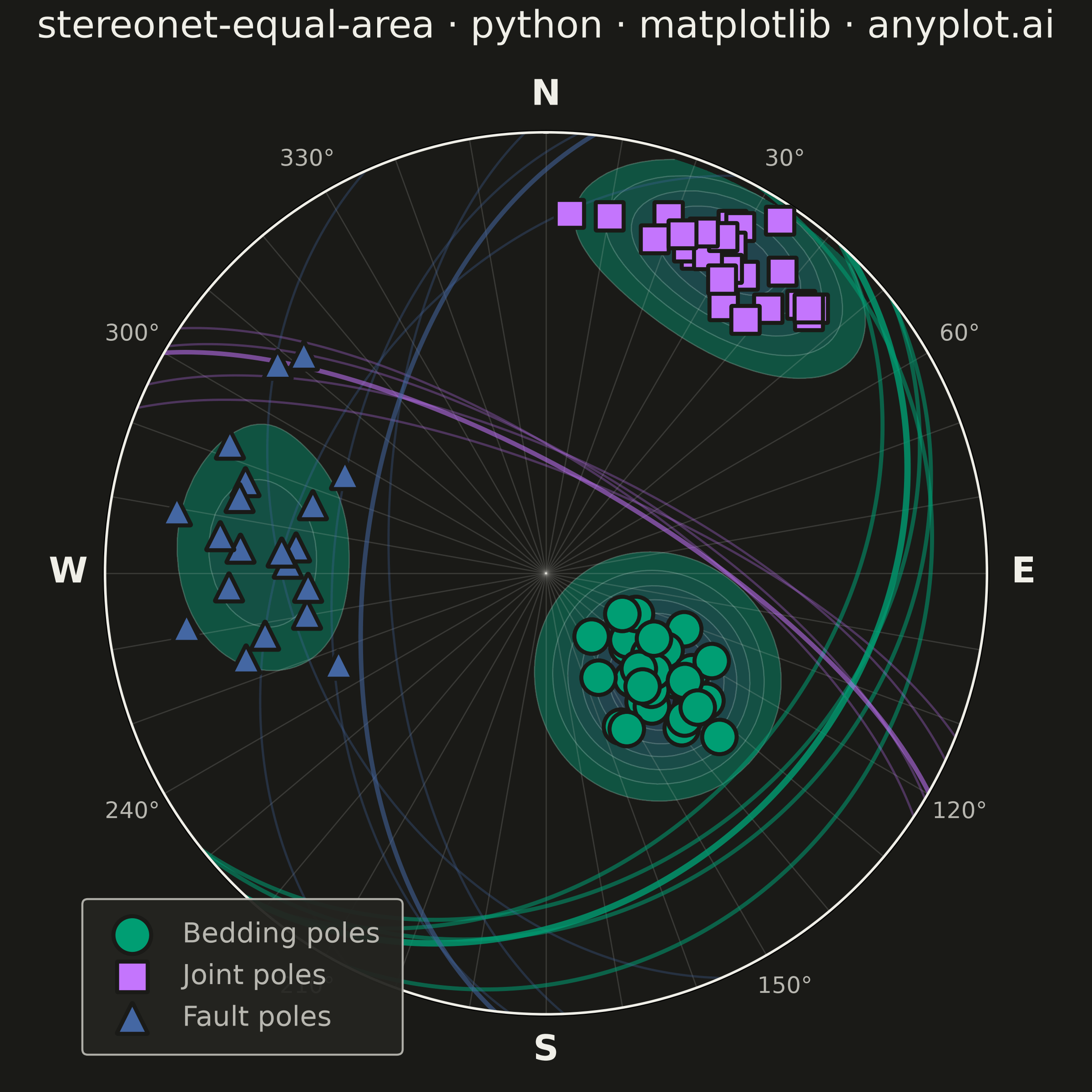
A Schmidt equal-area (lower-hemisphere) stereographic projection for plotting geological structural data. Great circles represent planar features (bedding, faults, joints) by their strike and dip, while poles to planes are plotted as points showing the orientation of the normal to each plane. Density contours highlight preferred orientations in clustered data. This is the standard projection used in structural geology for analyzing fabric elements and kinematic indicators.
""" anyplot.ai
stereonet-equal-area: Structural Geology Stereonet (Equal-Area Projection)
Library: matplotlib 3.11.0 | Python 3.13.14
Quality: 91/100 | Updated: 2026-06-16
"""

import os

import matplotlib.patheffects as pe
import matplotlib.pyplot as plt
import numpy as np
from matplotlib.collections import LineCollection
from matplotlib.colors import LinearSegmentedColormap


# Theme-adaptive chrome (see prompts/default-style-guide.md "Theme-adaptive Chrome")
THEME = os.getenv("ANYPLOT_THEME", "light")
PAGE_BG = "#FAF8F1" if THEME == "light" else "#1A1A17"
ELEVATED_BG = "#FFFDF6" if THEME == "light" else "#242420"
INK = "#1A1A17" if THEME == "light" else "#F0EFE8"
INK_SOFT = "#4A4A44" if THEME == "light" else "#B8B7B0"
INK_MUTED = "#6B6A63" if THEME == "light" else "#A8A79F"

# Imprint palette — first series is brand green; geological feature types are abstract
# so the canonical order applies (Bedding is the primary focus and keeps slot 1).
BEDDING = "#009E73"  # Imprint position 1 — brand green, primary feature
JOINT = "#C475FD"  # Imprint position 2 — lavender
FAULT = "#4467A3"  # Imprint position 3 — blue
# Single-polarity density → imprint_seq (brand green → blue), the only allowed sequential cmap
imprint_seq = LinearSegmentedColormap.from_list("imprint_seq", ["#009E73", "#4467A3"])

# Data - structural geology field measurements (strike/dip format)
np.random.seed(42)

bedding_strike = np.random.normal(45, 12, 30) % 360
bedding_dip = np.clip(np.random.normal(30, 8, 30), 2, 88)

joint_strike = np.random.normal(300, 10, 25) % 360
joint_dip = np.clip(np.random.normal(72, 7, 25), 2, 88)

fault_strike = np.random.normal(185, 15, 20) % 360
fault_dip = np.clip(np.random.normal(58, 10, 20), 2, 88)

datasets = {
    "Bedding": (bedding_strike, bedding_dip),
    "Joint": (joint_strike, joint_dip),
    "Fault": (fault_strike, fault_dip),
}
all_strikes = np.concatenate([bedding_strike, joint_strike, fault_strike])
all_dips = np.concatenate([bedding_dip, joint_dip, fault_dip])
feature_types = ["Bedding"] * 30 + ["Joint"] * 25 + ["Fault"] * 20

# Visual hierarchy: Bedding is the primary focus (larger markers, bolder great circles)
colors = {"Bedding": BEDDING, "Joint": JOINT, "Fault": FAULT}
markers = {"Bedding": "o", "Joint": "s", "Fault": "^"}
pole_sizes = {"Bedding": 170, "Joint": 110, "Fault": 110}
gc_alpha = {"Bedding": 0.55, "Joint": 0.30, "Fault": 0.30}
gc_lw = {"Bedding": 1.6, "Joint": 0.9, "Fault": 0.9}

# Poles to planes in equal-area (Schmidt) projection
pole_trend_rad = np.deg2rad((all_strikes + 90) % 360)
pole_r = np.sqrt(2) * np.sin(np.deg2rad(all_dips) / 2)

# Pole unit vectors on the lower hemisphere (East, North, Down) for density estimation
pole_colat = np.deg2rad(all_dips)
pole_vx = np.sin(pole_colat) * np.sin(pole_trend_rad)
pole_vy = np.sin(pole_colat) * np.cos(pole_trend_rad)
pole_vz = np.cos(pole_colat)

# Plot — square canvas (6 x 6 in @ 400 dpi = 2400 x 2400 px)
fig = plt.figure(figsize=(6, 6), dpi=400, facecolor=PAGE_BG)
ax = fig.add_subplot(111, projection="polar")
ax.set_theta_zero_location("N")
ax.set_theta_direction(-1)
ax.set_facecolor(PAGE_BG)

# Density contours from a spherical Gaussian kernel over the pole data
theta_grid = np.linspace(0, 2 * np.pi, 150)
r_grid = np.linspace(0.02, 0.98, 75)
THETA, R = np.meshgrid(theta_grid, r_grid)
colat_grid = 2 * np.arcsin(np.clip(R / np.sqrt(2), 0, 1))
gx = np.sin(colat_grid) * np.sin(THETA)
gy = np.sin(colat_grid) * np.cos(THETA)
gz = np.cos(colat_grid)

sigma = 0.20
Z = np.zeros(THETA.shape)
for j in range(len(all_dips)):
    cos_dist = gx * pole_vx[j] + gy * pole_vy[j] + gz * pole_vz[j]
    Z += np.exp(-(np.arccos(np.clip(cos_dist, -1, 1)) ** 2) / (2 * sigma**2))

# Threshold the lowest band so only clustered orientations are tinted (not the whole disk)
levels = np.linspace(Z.max() * 0.22, Z.max(), 8)
ax.contourf(THETA, R, Z, levels=levels, cmap=imprint_seq, alpha=0.45, zorder=1)
ax.contour(THETA, R, Z, levels=levels, colors=INK_MUTED, alpha=0.30, linewidths=0.5, zorder=1)

# Great circles per feature type — bold mean plane + a representative subset.
# Vectorised inline over the small set so no helper function is needed.
t_param = np.linspace(0, np.pi, 180)
for feat, (strikes, dips) in datasets.items():
    color = colors[feat]
    mean_strike = (
        np.degrees(np.arctan2(np.mean(np.sin(np.deg2rad(strikes))), np.mean(np.cos(np.deg2rad(strikes))))) % 360
    )
    mean_dip = np.mean(dips)
    idx = np.linspace(0, len(strikes) - 1, 4, dtype=int)
    gc_strikes = np.concatenate([[mean_strike], strikes[idx]])
    gc_dips = np.concatenate([[mean_dip], dips[idx]])

    alpha = np.deg2rad(gc_strikes)[:, None]
    delta = np.deg2rad(gc_dips)[:, None]
    px = np.cos(t_param) * np.sin(alpha) + np.sin(t_param) * np.cos(alpha) * np.cos(delta)
    py = np.cos(t_param) * np.cos(alpha) - np.sin(t_param) * np.sin(alpha) * np.cos(delta)
    pz = np.sin(t_param) * np.sin(delta)
    trend = np.arctan2(px, py)
    plunge = np.arctan2(pz, np.hypot(px, py))
    r_gc = np.sqrt(2) * np.sin((np.pi / 2 - plunge) / 2)

    # Mean plane (bold), then representative planes (thin)
    ax.plot(trend[0], r_gc[0], color=color, alpha=gc_alpha[feat] + 0.25, linewidth=gc_lw[feat] + 0.9, zorder=3)
    segments = [np.column_stack([trend[i], r_gc[i]]) for i in range(1, len(gc_strikes))]
    ax.add_collection(LineCollection(segments, colors=color, alpha=gc_alpha[feat], linewidths=gc_lw[feat], zorder=2))

# Poles as scatter points with distinct markers per feature type
for feat in colors:
    mask = np.array([ft == feat for ft in feature_types])
    ax.scatter(
        pole_trend_rad[mask],
        pole_r[mask],
        c=colors[feat],
        s=pole_sizes[feat],
        marker=markers[feat],
        edgecolors=PAGE_BG,
        linewidth=1.0,
        label=f"{feat} poles",
        zorder=5,
        path_effects=[pe.withStroke(linewidth=2.2, foreground=PAGE_BG)],
    )

# Style — perimeter degree ticks every 10°, labels at 30° with bold cardinals
ax.set_rlim(0, 1)
ax.set_rticks([])
theta_ticks = np.arange(0, 360, 10)
ax.set_xticks(np.deg2rad(theta_ticks))
tick_labels = []
for d in theta_ticks:
    if d == 0:
        tick_labels.append("N")
    elif d == 90:
        tick_labels.append("E")
    elif d == 180:
        tick_labels.append("S")
    elif d == 270:
        tick_labels.append("W")
    elif d % 30 == 0:
        tick_labels.append(f"{d}°")
    else:
        tick_labels.append("")
ax.set_xticklabels(tick_labels, fontsize=9, color=INK_SOFT)

# Emphasise the cardinal direction labels
for label in ax.get_xticklabels():
    if label.get_text() in ("N", "E", "S", "W"):
        label.set_fontsize(14)
        label.set_fontweight("bold")
        label.set_color(INK)
        label.set_path_effects([pe.withStroke(linewidth=2, foreground=PAGE_BG)])
ax.grid(True, alpha=0.15, linewidth=0.5, color=INK)

# Primitive circle (the horizontal plane)
circle_theta = np.linspace(0, 2 * np.pi, 300)
ax.plot(circle_theta, np.ones_like(circle_theta), color=INK, linewidth=2.0, zorder=4)

# Legend positioned clear of the perimeter ticks
legend = ax.legend(
    loc="lower left",
    bbox_to_anchor=(-0.04, -0.06),
    fontsize=11,
    framealpha=0.95,
    fancybox=True,
    markerscale=1.1,
    borderpad=0.8,
)
legend.get_frame().set_facecolor(ELEVATED_BG)
legend.get_frame().set_edgecolor(INK_SOFT)
legend.get_frame().set_linewidth(0.8)
for text in legend.get_texts():
    text.set_color(INK_SOFT)

ax.set_title(
    "stereonet-equal-area · python · matplotlib · anyplot.ai", fontsize=15, fontweight="medium", pad=16, color=INK
)

# Save — square canvas, no bbox_inches="tight" (it would shave the canvas off-target)
fig.subplots_adjust(left=0.07, right=0.93, top=0.88, bottom=0.07)
plt.savefig(f"plot-{THEME}.png", dpi=400, facecolor=PAGE_BG)
Runnable source as JSON, for any HTTP client: https://api.anyplot.ai/specs/stereonet-equal-area/matplotlib/code. Any spec id and library id listed in llms-full.txt fit the same URL shape; every URL below is complete and callable.
{
  "spec_id": "stereonet-equal-area",
  "language": "python",
  "library": "matplotlib",
  "page": "https://anyplot.ai/stereonet-equal-area/python/matplotlib",
  "hub": "https://anyplot.ai/stereonet-equal-area",
  "code_json": "https://api.anyplot.ai/specs/stereonet-equal-area/matplotlib/code",
  "spec_json": "https://api.anyplot.ai/specs/stereonet-equal-area",
  "render_light_png": "https://storage.googleapis.com/anyplot-images/plots/stereonet-equal-area/python/matplotlib/plot-light.png",
  "render_dark_png": "https://storage.googleapis.com/anyplot-images/plots/stereonet-equal-area/python/matplotlib/plot-dark.png",
  "quality_score": 91.0,
  "license": "MIT",
  "guide": "https://anyplot.ai/llms.txt"
}
Part of Structural Geology Stereonet (Equal-Area Projection) on anyplot.ai.