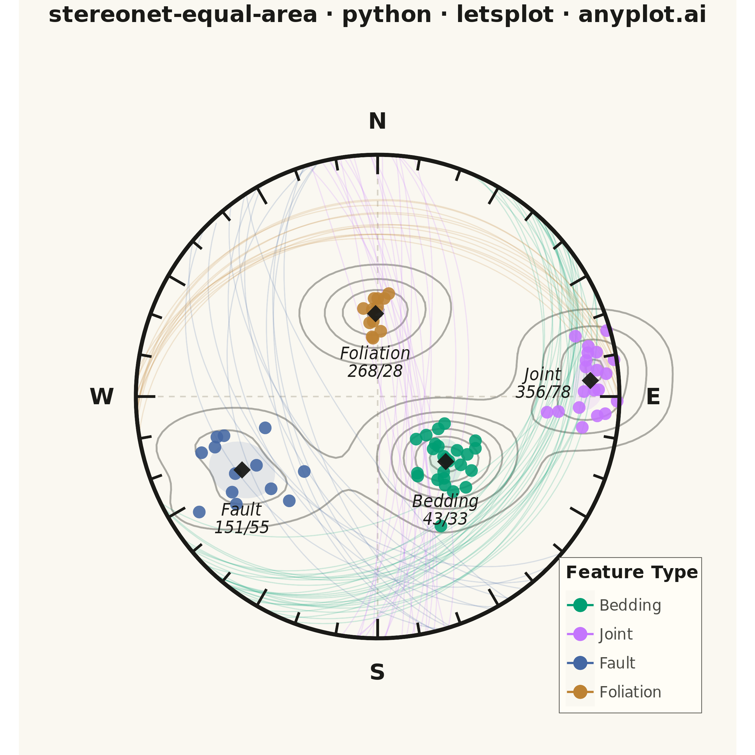
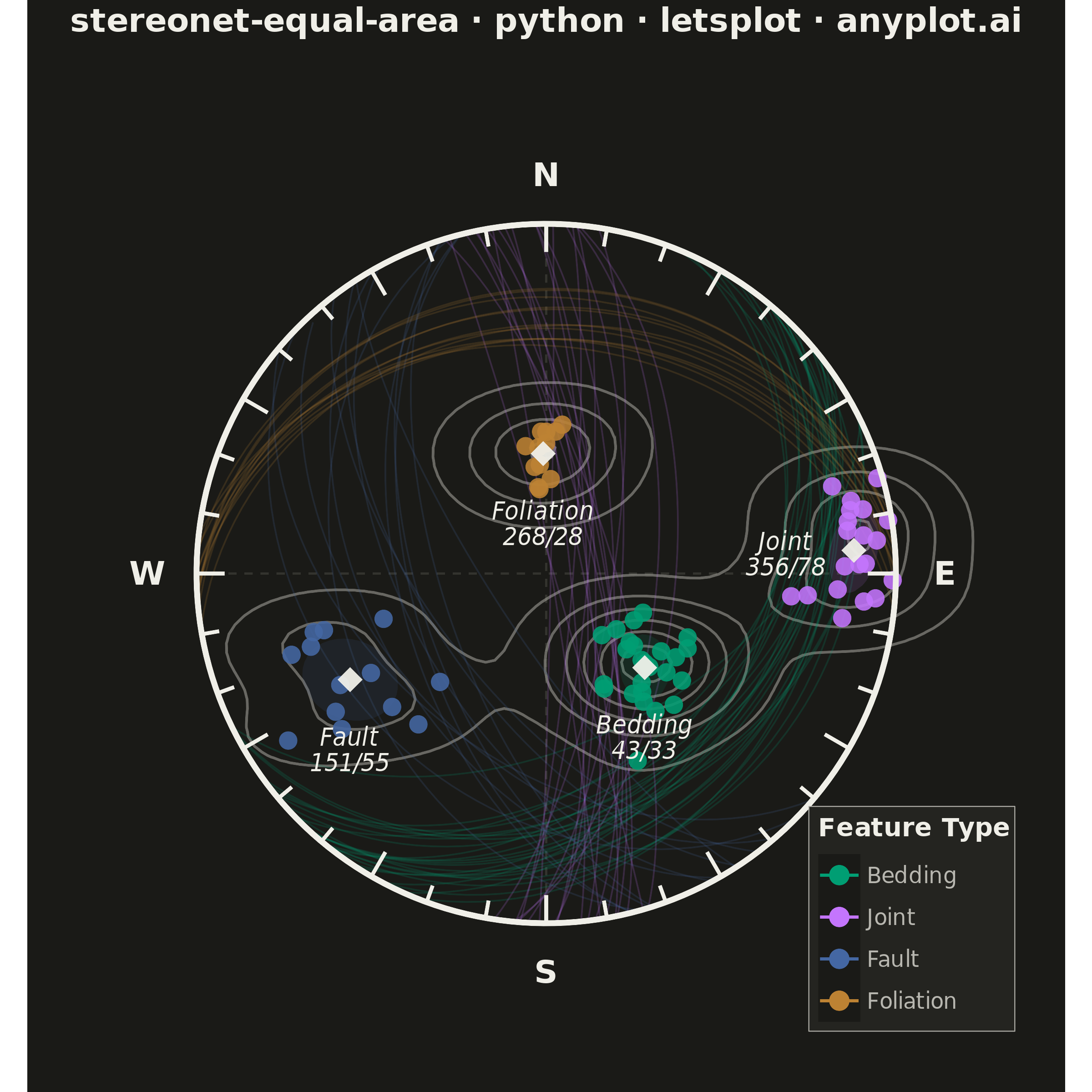
A Schmidt equal-area (lower-hemisphere) stereographic projection for plotting geological structural data. Great circles represent planar features (bedding, faults, joints) by their strike and dip, while poles to planes are plotted as points showing the orientation of the normal to each plane. Density contours highlight preferred orientations in clustered data. This is the standard projection used in structural geology for analyzing fabric elements and kinematic indicators.
""" anyplot.ai
stereonet-equal-area: Structural Geology Stereonet (Equal-Area Projection)
Library: letsplot 4.10.1 | Python 3.13.13
Quality: 88/100 | Updated: 2026-06-16
"""

import os

import numpy as np
import pandas as pd
from lets_plot import (
    LetsPlot,
    aes,
    coord_fixed,
    element_blank,
    element_rect,
    element_text,
    geom_density2d,
    geom_path,
    geom_point,
    geom_polygon,
    geom_segment,
    geom_text,
    ggplot,
    ggsize,
    labs,
    layer_tooltips,
    scale_color_manual,
    scale_fill_manual,
    scale_x_continuous,
    scale_y_continuous,
    theme,
)
from lets_plot.export import ggsave


LetsPlot.setup_html()

# Theme-adaptive chrome (Imprint design tokens)
THEME = os.getenv("ANYPLOT_THEME", "light")
PAGE_BG = "#FAF8F1" if THEME == "light" else "#1A1A17"
ELEVATED_BG = "#FFFDF6" if THEME == "light" else "#242420"
INK = "#1A1A17" if THEME == "light" else "#F0EFE8"
INK_SOFT = "#4A4A44" if THEME == "light" else "#B8B7B0"
INK_MUTED = "#6B6A63" if THEME == "light" else "#A8A79F"
RULE = "#D8D4C8" if THEME == "light" else "#33332E"

# Imprint categorical palette — first series ALWAYS #009E73
# 4 abstract structural-feature classes → canonical order 1→4
IMPRINT_PALETTE = ["#009E73", "#C475FD", "#4467A3", "#BD8233"]

# Data - Field measurements from a structural geology mapping campaign
np.random.seed(42)

# Bedding planes (NE strike ~045, moderate dip ~35° SE)
n_bedding = 25
bedding_strike = np.random.normal(45, 12, n_bedding) % 360
bedding_dip = np.clip(np.random.normal(35, 8, n_bedding), 5, 85)

# Joint set (N-S striking ~000, steep dip ~78° W)
n_joints = 20
joints_strike = np.random.normal(355, 10, n_joints) % 360
joints_dip = np.clip(np.random.normal(78, 7, n_joints), 10, 89)

# Faults (NW-SE striking ~150, moderate-steep dip ~60°)
n_faults = 13
faults_strike = np.random.uniform(130, 170, n_faults)
faults_dip = np.clip(np.random.normal(60, 12, n_faults), 10, 89)

# Foliation (E-W strike ~270, gentle dip ~25° N)
n_foliation = 12
foliation_strike = np.random.normal(270, 8, n_foliation) % 360
foliation_dip = np.clip(np.random.normal(25, 6, n_foliation), 5, 60)

strikes = np.concatenate([bedding_strike, joints_strike, faults_strike, foliation_strike])
dips = np.concatenate([bedding_dip, joints_dip, faults_dip, foliation_dip])
feature_types = ["Bedding"] * n_bedding + ["Joint"] * n_joints + ["Fault"] * n_faults + ["Foliation"] * n_foliation

# Equal-area (Schmidt net) lower-hemisphere projection
strike_rad = np.radians(strikes)
dip_rad = np.radians(dips)
dip_dir_rad = strike_rad + np.pi / 2

# Pole 3D coordinates (lower hemisphere normal to each plane)
pole_x_3d = np.sin(dip_rad) * np.sin(dip_dir_rad)
pole_y_3d = np.sin(dip_rad) * np.cos(dip_dir_rad)
pole_z_3d = -np.cos(dip_rad)

# Lambert azimuthal equal-area projection
pole_scale = 1.0 / np.sqrt(1.0 - pole_z_3d)
pole_x = pole_x_3d * pole_scale
pole_y = pole_y_3d * pole_scale

poles_df = pd.DataFrame(
    {
        "x": pole_x,
        "y": pole_y,
        "feature_type": feature_types,
        "strike": [f"{s:.0f}°" for s in strikes],
        "dip": [f"{d:.0f}°" for d in dips],
    }
)

# Great circle paths for each plane
gc_rows = []
alphas = np.linspace(0, np.pi, 60)
cos_a = np.cos(alphas)
sin_a = np.sin(alphas)

for i in range(len(strikes)):
    s = strike_rad[i]
    d = dip_rad[i]
    dd = dip_dir_rad[i]
    sv_x, sv_y = np.sin(s), np.cos(s)
    dv_x = np.cos(d) * np.sin(dd)
    dv_y = np.cos(d) * np.cos(dd)
    dv_z = -np.sin(d)
    px = cos_a * sv_x + sin_a * dv_x
    py = cos_a * sv_y + sin_a * dv_y
    pz = sin_a * dv_z
    sc = 1.0 / np.sqrt(1.0 - pz)
    gx = px * sc
    gy = py * sc
    # Clip to unit circle boundary
    r2 = gx**2 + gy**2
    mask_inside = r2 <= 1.0
    gx_clip = gx[mask_inside]
    gy_clip = gy[mask_inside]
    for j in range(len(gx_clip)):
        gc_rows.append({"x": gx_clip[j], "y": gy_clip[j], "group": i, "feature_type": feature_types[i]})

gc_df = pd.DataFrame(gc_rows)

# Primitive circle (outer boundary)
theta = np.linspace(0, 2 * np.pi, 200)
circle_df = pd.DataFrame({"x": np.cos(theta), "y": np.sin(theta)})

# Annular mask — covers any density bleed outside the primitive circle with the
# page background so the stereonet stays cleanly bounded (built as fan quads
# between r=1 and r=1.6, one filled polygon per angular segment).
mask_rows = []
n_seg = 180
for k in range(n_seg):
    a0 = 2 * np.pi * k / n_seg
    a1 = 2 * np.pi * (k + 1) / n_seg
    inner0 = (np.cos(a0), np.sin(a0))
    inner1 = (np.cos(a1), np.sin(a1))
    outer0 = (1.6 * np.cos(a0), 1.6 * np.sin(a0))
    outer1 = (1.6 * np.cos(a1), 1.6 * np.sin(a1))
    for vx, vy in [inner0, outer0, outer1, inner1]:
        mask_rows.append({"x": vx, "y": vy, "group": k})
mask_df = pd.DataFrame(mask_rows)

# Tick marks every 10° (longer every 30°)
tick_rows = []
for deg in range(0, 360, 10):
    rad = np.radians(deg)
    inner_r = 0.95 if deg % 30 != 0 else 0.92
    tick_rows.append({"x": np.sin(rad) * inner_r, "y": np.cos(rad) * inner_r, "xend": np.sin(rad), "yend": np.cos(rad)})
tick_df = pd.DataFrame(tick_rows)

# Reference cross lines (N-S, E-W)
ref_df = pd.DataFrame(
    [{"x": 0, "y": -1, "xend": 0, "yend": 1, "group": 0}, {"x": -1, "y": 0, "xend": 1, "yend": 0, "group": 1}]
)

# Cardinal direction labels
cardinal_positions = [(0, 1.14, "N"), (1.14, 0, "E"), (0, -1.14, "S"), (-1.14, 0, "W")]
label_df = pd.DataFrame(
    {
        "x": [c[0] for c in cardinal_positions],
        "y": [c[1] for c in cardinal_positions],
        "label": [c[2] for c in cardinal_positions],
    }
)

# Mean pole annotations and confidence ellipses per feature type
mean_annotations = []
ellipse_rows = []
for idx, ft in enumerate(["Bedding", "Joint", "Fault", "Foliation"]):
    mask = np.array(feature_types) == ft
    mx = pole_x[mask].mean()
    my = pole_y[mask].mean()
    # Circular mean for strike (handles wraparound at 0/360°)
    s_rad = np.radians(strikes[mask])
    ms = np.degrees(np.arctan2(np.sin(s_rad).mean(), np.cos(s_rad).mean())) % 360
    md = dips[mask].mean()
    # Smart label nudge: push outward from cluster centroid, away from cardinal labels
    nudge_x, nudge_y = 0.0, -0.20
    for cx, cy, _ in cardinal_positions:
        dist = np.sqrt((mx - cx) ** 2 + (my - cy) ** 2)
        if dist < 0.45:
            # Push label away from the nearby cardinal direction, toward the centre
            dx, dy = mx - cx, my - cy
            norm = max(np.sqrt(dx**2 + dy**2), 0.01)
            nudge_x = dx / norm * 0.20
            nudge_y = dy / norm * 0.20 - 0.06
    mean_annotations.append(
        {"x": mx, "y": my, "label": f"{ft}\n{ms:.0f}/{md:.0f}", "nudge_x": nudge_x, "nudge_y": nudge_y}
    )
    # Confidence ellipse (1-sigma) around each cluster
    px_ft = pole_x[mask]
    py_ft = pole_y[mask]
    cov = np.cov(px_ft, py_ft)
    eigvals, eigvecs = np.linalg.eigh(cov)
    angle = np.arctan2(eigvecs[1, 1], eigvecs[0, 1])
    t = np.linspace(0, 2 * np.pi, 40)
    ex = np.sqrt(eigvals[1]) * np.cos(t)
    ey = np.sqrt(eigvals[0]) * np.sin(t)
    rx = mx + ex * np.cos(angle) - ey * np.sin(angle)
    ry = my + ex * np.sin(angle) + ey * np.cos(angle)
    for j in range(len(t)):
        ellipse_rows.append({"x": rx[j], "y": ry[j], "group": idx, "feature_type": ft})

ellipse_df = pd.DataFrame(ellipse_rows)
mean_df = pd.DataFrame(mean_annotations)

# Tooltips for poles showing strike/dip
pole_tooltips = layer_tooltips().line("@feature_type").line("Strike: @strike").line("Dip: @dip")

# Build individual mean label layers to handle per-label nudge offsets
mean_label_layers = []
for _, row in mean_df.iterrows():
    single_df = pd.DataFrame([{"x": row["x"], "y": row["y"], "label": row["label"]}])
    mean_label_layers.append(
        geom_text(
            aes(x="x", y="y", label="label"),
            data=single_df,
            size=7,
            color=INK,
            nudge_x=row["nudge_x"],
            nudge_y=row["nudge_y"],
            fontface="italic",
            show_legend=False,
        )
    )

# Plot
plot = (
    ggplot()
    # Reference cross lines
    + geom_segment(aes(x="x", y="y", xend="xend", yend="yend"), data=ref_df, color=RULE, size=0.5, linetype="dashed")
    # Density contours (Kamb-style preferred-orientation clustering)
    + geom_density2d(
        aes(x="x", y="y"),
        data=poles_df,
        color=INK_MUTED,
        alpha=0.55,
        size=0.6,
        bins=6,
        kernel="gaussian",
        adjust=0.8,
        show_legend=False,
    )
    # Great circles
    + geom_path(aes(x="x", y="y", group="group", color="feature_type"), data=gc_df, size=0.35, alpha=0.18)
    # Confidence ellipses around each cluster
    + geom_polygon(
        aes(x="x", y="y", group="group", fill="feature_type"), data=ellipse_df, alpha=0.12, size=0, show_legend=False
    )
    # Poles to planes with tooltips
    + geom_point(aes(x="x", y="y", color="feature_type"), data=poles_df, size=4.5, alpha=0.88, tooltips=pole_tooltips)
    # Mean pole markers (diamond shape)
    + geom_point(aes(x="x", y="y"), data=mean_df, size=9, shape=18, color=INK, alpha=0.95, show_legend=False)
)

# Add per-label mean annotation layers
for layer in mean_label_layers:
    plot = plot + layer

plot = (
    plot
    # Annular mask hides density bleed outside the primitive circle
    + geom_polygon(aes(x="x", y="y", group="group"), data=mask_df, fill=PAGE_BG, color=PAGE_BG, size=0)
    # Primitive circle
    + geom_path(aes(x="x", y="y"), data=circle_df, color=INK, size=1.4)
    # Tick marks
    + geom_segment(aes(x="x", y="y", xend="xend", yend="yend"), data=tick_df, color=INK, size=0.9)
    # Cardinal labels
    + geom_text(aes(x="x", y="y", label="label"), data=label_df, size=9, color=INK, fontface="bold")
    # Color scale (Imprint palette)
    + scale_color_manual(values=IMPRINT_PALETTE, name="Feature Type")
    + scale_fill_manual(values=IMPRINT_PALETTE)
    + coord_fixed()
    + scale_x_continuous(limits=[-1.32, 1.32])
    + scale_y_continuous(limits=[-1.32, 1.32])
    + labs(title="stereonet-equal-area · python · letsplot · anyplot.ai")
    + theme(
        plot_title=element_text(size=18, hjust=0.5, face="bold", color=INK, margin=[0, 0, 12, 0]),
        legend_title=element_text(size=14, face="bold", color=INK),
        legend_text=element_text(size=12, color=INK_SOFT),
        legend_position=[0.86, 0.16],
        legend_justification=[0.5, 0.5],
        legend_background=element_rect(fill=ELEVATED_BG, color=INK_SOFT, size=0.5),
        axis_title=element_blank(),
        axis_text=element_blank(),
        axis_ticks=element_blank(),
        axis_line=element_blank(),
        panel_grid=element_blank(),
        plot_background=element_rect(fill=PAGE_BG, color=PAGE_BG),
        panel_background=element_rect(fill=PAGE_BG, color=PAGE_BG),
    )
    + ggsize(600, 600)
)

ggsave(plot, f"plot-{THEME}.png", path=".", scale=4)
ggsave(plot, f"plot-{THEME}.html", path=".")
Runnable source as JSON, for any HTTP client: https://api.anyplot.ai/specs/stereonet-equal-area/letsplot/code. Any spec id and library id listed in llms-full.txt fit the same URL shape; every URL below is complete and callable.
{
  "spec_id": "stereonet-equal-area",
  "language": "python",
  "library": "letsplot",
  "page": "https://anyplot.ai/stereonet-equal-area/python/letsplot",
  "hub": "https://anyplot.ai/stereonet-equal-area",
  "code_json": "https://api.anyplot.ai/specs/stereonet-equal-area/letsplot/code",
  "spec_json": "https://api.anyplot.ai/specs/stereonet-equal-area",
  "render_light_png": "https://storage.googleapis.com/anyplot-images/plots/stereonet-equal-area/python/letsplot/plot-light.png",
  "render_dark_png": "https://storage.googleapis.com/anyplot-images/plots/stereonet-equal-area/python/letsplot/plot-dark.png",
  "interactive_light_html": "https://storage.googleapis.com/anyplot-images/plots/stereonet-equal-area/python/letsplot/plot-light.html",
  "interactive_dark_html": "https://storage.googleapis.com/anyplot-images/plots/stereonet-equal-area/python/letsplot/plot-dark.html",
  "quality_score": 88.0,
  "license": "MIT",
  "guide": "https://anyplot.ai/llms.txt"
}
Part of Structural Geology Stereonet (Equal-Area Projection) on anyplot.ai.