Basic Swarm Plot — D3.js

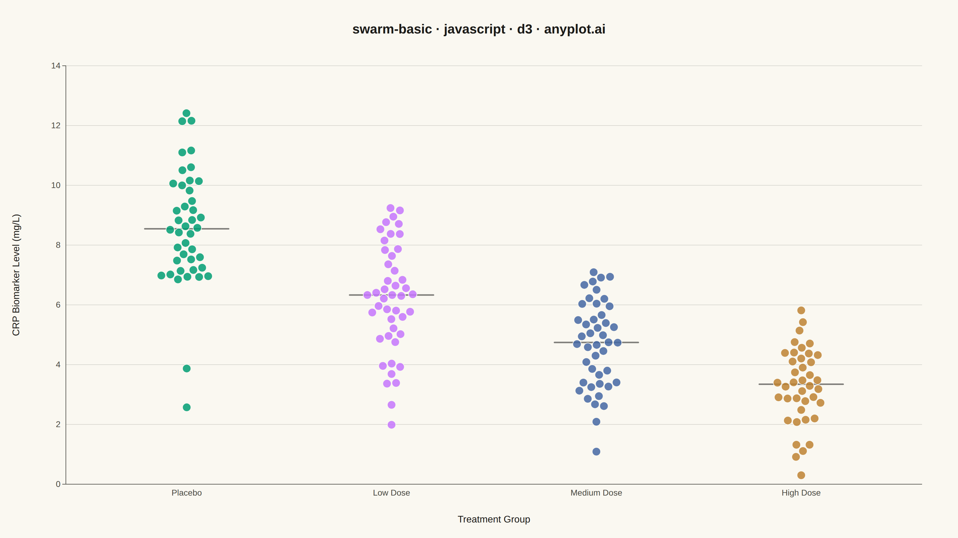
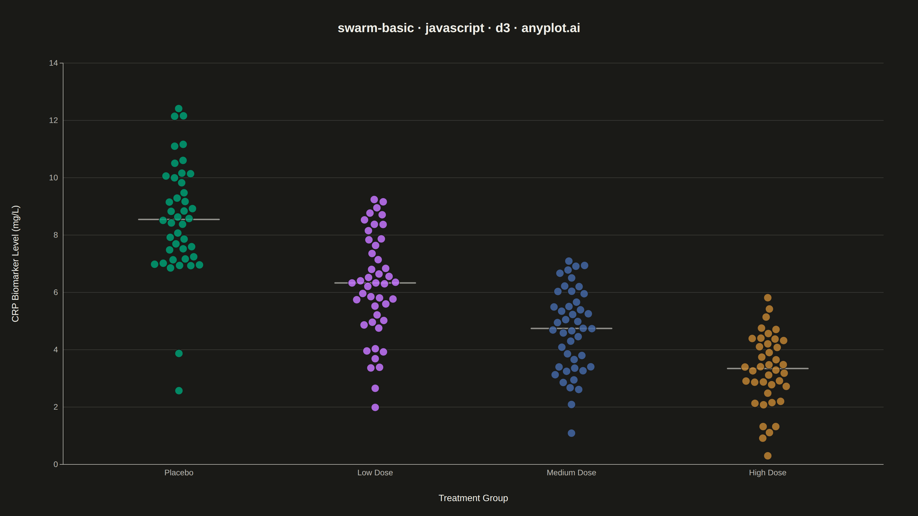
A swarm plot (beeswarm plot) displays individual data points for categorical comparisons, with points spread horizontally to avoid overlap. This reveals the full distribution shape and density while preserving exact values - combining the benefits of strip plots (individual points) and violin plots (density visualization). Ideal when you need to see every observation rather than just summary statistics.
JavaScript source (D3.js)

// anyplot.ai
// swarm-basic: Basic Swarm Plot
// Library: d3 7.9.0 | JavaScript 22.23.1
// Quality: 92/100 | Created: 2026-07-26

const t = window.ANYPLOT_TOKENS;
const { width, height } = window.ANYPLOT_SIZE;
const margin = { top: 110, right: 60, bottom: 90, left: 110 };
const iw = width - margin.left - margin.right;
const ih = height - margin.top - margin.bottom;

// --- Data (in-memory, deterministic, fixed-seed LCG) ------------------------
let seed = 42;
function lcgUniform() {
  seed = (seed * 1664525 + 1013904223) % 4294967296;
  return seed / 4294967296;
}
function gaussian(mean, sd) {
  const u1 = Math.max(lcgUniform(), 1e-9);
  const u2 = lcgUniform();
  const z = Math.sqrt(-2 * Math.log(u1)) * Math.cos(2 * Math.PI * u2);
  return mean + z * sd;
}

const groups = [
  { category: "Placebo", mean: 8.2, sd: 2.1, n: 42 },
  { category: "Low Dose", mean: 6.4, sd: 1.9, n: 45 },
  { category: "Medium Dose", mean: 4.6, sd: 1.7, n: 44 },
  { category: "High Dose", mean: 3.1, sd: 1.4, n: 40 },
];

const data = [];
for (const grp of groups) {
  for (let i = 0; i < grp.n; i++) {
    data.push({ category: grp.category, value: Math.max(0.3, gaussian(grp.mean, grp.sd)) });
  }
}
const categories = groups.map((grp) => grp.category);

// --- Scales -------------------------------------------------------------
// Domain hugs the data range (not zero-anchored) — a swarm reads individual
// values, not magnitude-from-zero, so a tight domain uses the canvas fully.
const dataMin = d3.min(data, (d) => d.value);
const dataMax = d3.max(data, (d) => d.value);
const pad = (dataMax - dataMin) * 0.08;
const x = d3.scaleBand().domain(categories).range([0, iw]).padding(0.18);
const y = d3
  .scaleLinear()
  .domain([Math.max(0, dataMin - pad), dataMax + pad])
  .nice()
  .range([ih, 0]);
const color = d3.scaleOrdinal().domain(categories).range(t.palette);

// --- Beeswarm layout (force simulation, settled synchronously) --------------
// `fy` pins each node's vertical position exactly to its value — only x is
// free, so the simulation resolves overlap purely by spreading horizontally
// (a `forceY` pull instead of a fixed `fy` lets collide drag points off the
// value line entirely, even clipping them off-canvas at high density).
const radius = 7;
const nodes = data.map((d) => ({
  ...d,
  targetX: x(d.category) + x.bandwidth() / 2,
  fy: y(d.value),
}));

const simulation = d3
  .forceSimulation(nodes)
  .force("x", d3.forceX((d) => d.targetX).strength(0.15))
  .force("collide", d3.forceCollide(radius + 0.6))
  .stop();
for (let i = 0; i < 300; i++) simulation.tick();

// Keep points within their own band so groups never bleed into neighbors.
for (const n of nodes) {
  const lo = x(n.category) + radius;
  const hi = x(n.category) + x.bandwidth() - radius;
  n.x = Math.min(hi, Math.max(lo, n.x));
}

// --- SVG mount ----------------------------------------------------------
const svg = d3.select("#container").append("svg").attr("width", width).attr("height", height);
const g = svg.append("g").attr("transform", `translate(${margin.left},${margin.top})`);

// --- Gridlines (y-axis only, subtle) -----------------------------------
g.append("g")
  .call(d3.axisLeft(y).ticks(6).tickSize(-iw).tickFormat(""))
  .call((sel) => sel.select(".domain").remove())
  .selectAll("line")
  .attr("stroke", t.grid);

// --- Median markers per category (drawn under the points) -------------------
const markerHalfWidth = 70;
for (const cat of categories) {
  const values = data.filter((d) => d.category === cat).map((d) => d.value);
  const median = d3.median(values);
  const cx = x(cat) + x.bandwidth() / 2;
  g.append("line")
    .attr("x1", cx - markerHalfWidth)
    .attr("x2", cx + markerHalfWidth)
    .attr("y1", y(median))
    .attr("y2", y(median))
    .attr("stroke", t.ink)
    .attr("stroke-width", 2.5)
    .attr("stroke-opacity", 0.55)
    .attr("stroke-linecap", "round");
}

// --- Points -------------------------------------------------------------
g.selectAll("circle")
  .data(nodes)
  .join("circle")
  .attr("cx", (d) => d.x)
  .attr("cy", (d) => d.y)
  .attr("r", radius)
  .attr("fill", (d) => color(d.category))
  .attr("fill-opacity", 0.85)
  .attr("stroke", t.pageBg)
  .attr("stroke-width", 1);

// --- Axes -----------------------------------------------------------------
const xAxis = g.append("g").attr("transform", `translate(0,${ih})`).call(d3.axisBottom(x).tickSizeOuter(0));
const yAxis = g.append("g").call(d3.axisLeft(y).ticks(6));
for (const ax of [xAxis, yAxis]) {
  ax.selectAll("text").attr("fill", t.inkSoft).style("font-size", "14px");
  ax.selectAll(".tick line").remove();
  ax.select(".domain").attr("stroke", t.inkSoft);
}

// --- Axis labels ------------------------------------------------------------
g.append("text")
  .attr("x", iw / 2)
  .attr("y", ih + 64)
  .attr("text-anchor", "middle")
  .attr("fill", t.ink)
  .style("font-size", "16px")
  .text("Treatment Group");

g.append("text")
  .attr("transform", "rotate(-90)")
  .attr("x", -ih / 2)
  .attr("y", -78)
  .attr("text-anchor", "middle")
  .attr("fill", t.ink)
  .style("font-size", "16px")
  .text("CRP Biomarker Level (mg/L)");

// --- Title --------------------------------------------------------------
svg
  .append("text")
  .attr("x", width / 2)
  .attr("y", 56)
  .attr("text-anchor", "middle")
  .attr("fill", t.ink)
  .style("font-size", "22px")
  .style("font-weight", "600")
  .text("swarm-basic · javascript · d3 · anyplot.ai");
Part of Basic Swarm Plot on anyplot.ai.
Basic Swarm Plot — D3.js

JavaScript source (D3.js)

Other implementations
