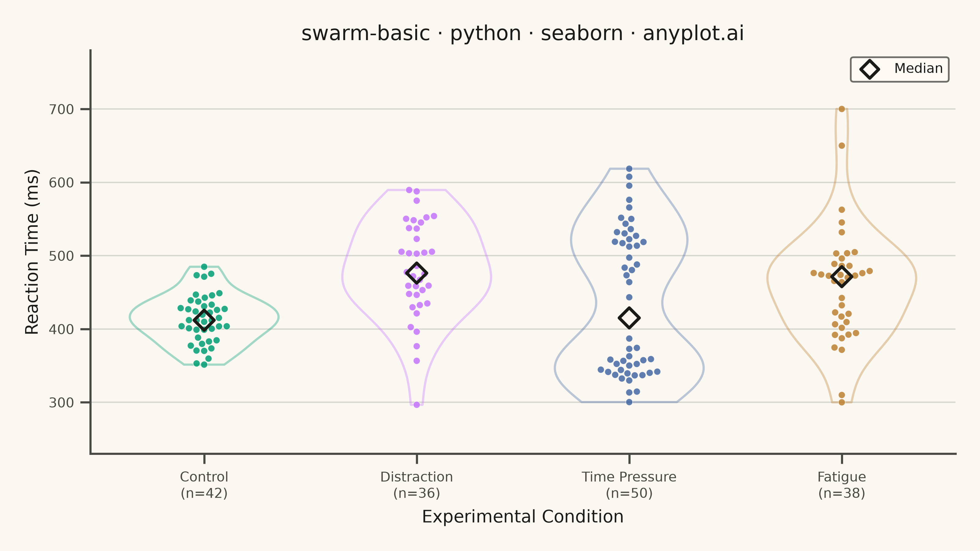
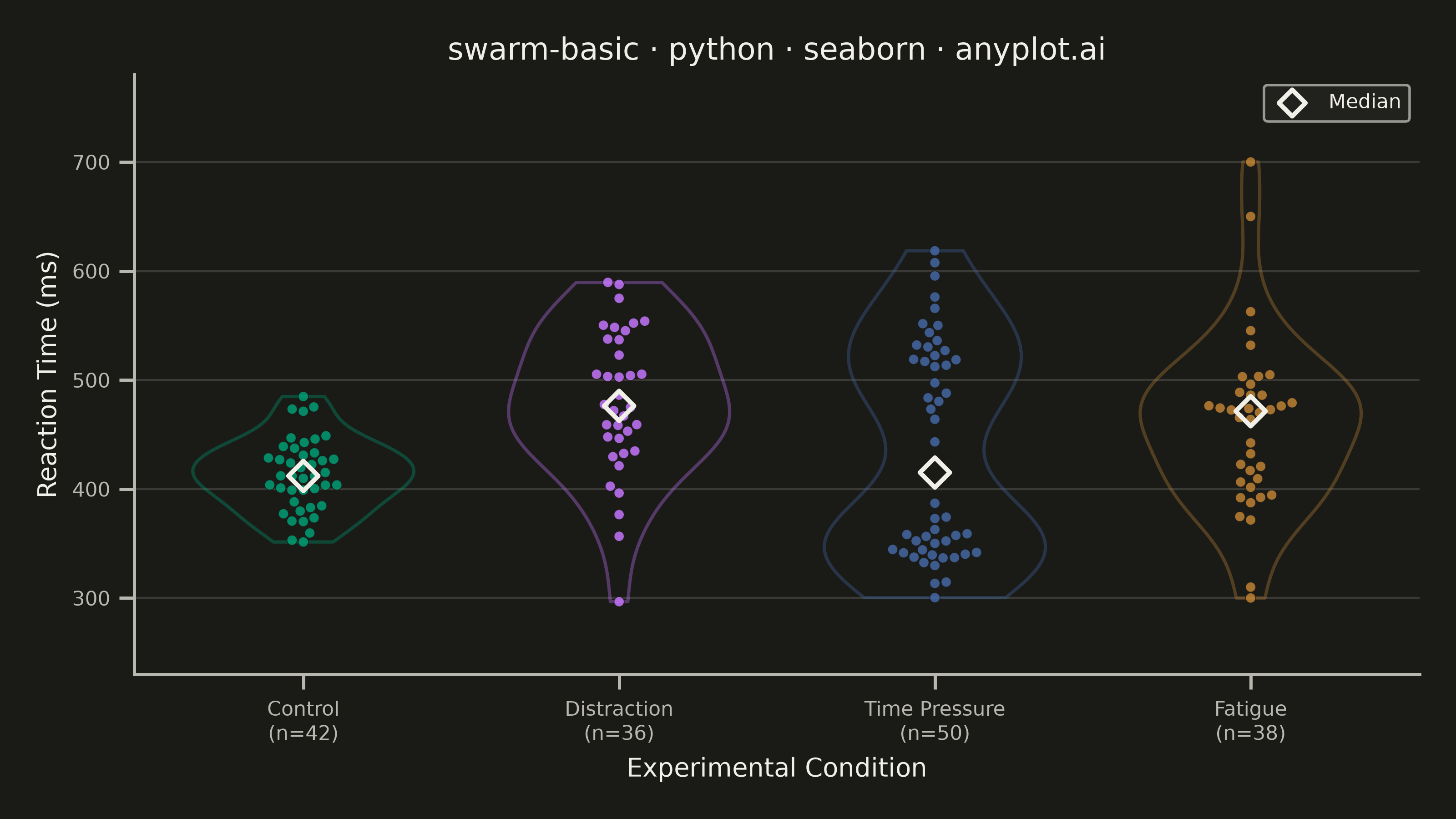
A swarm plot (beeswarm plot) displays individual data points for categorical comparisons, with points spread horizontally to avoid overlap. This reveals the full distribution shape and density while preserving exact values - combining the benefits of strip plots (individual points) and violin plots (density visualization). Ideal when you need to see every observation rather than just summary statistics.
""" anyplot.ai
swarm-basic: Basic Swarm Plot
Library: seaborn 0.13.2 | Python 3.13.14
Quality: 94/100 | Updated: 2026-07-26
"""

import os

import matplotlib.pyplot as plt
import numpy as np
import pandas as pd
import seaborn as sns


# Theme tokens (see prompts/default-style-guide.md "Theme-adaptive Chrome")
THEME = os.getenv("ANYPLOT_THEME", "light")
PAGE_BG = "#FAF8F1" if THEME == "light" else "#1A1A17"
ELEVATED_BG = "#FFFDF6" if THEME == "light" else "#242420"
INK = "#1A1A17" if THEME == "light" else "#F0EFE8"
INK_SOFT = "#4A4A44" if THEME == "light" else "#B8B7B0"

# Imprint categorical palette — first series always #009E73
IMPRINT_PALETTE = ["#009E73", "#C475FD", "#4467A3", "#BD8233"]

sns.set_theme(
    style="ticks",
    rc={
        "figure.facecolor": PAGE_BG,
        "axes.facecolor": PAGE_BG,
        "axes.edgecolor": INK_SOFT,
        "axes.labelcolor": INK,
        "text.color": INK,
        "xtick.color": INK_SOFT,
        "ytick.color": INK_SOFT,
        "grid.color": INK,
        "grid.alpha": 0.15,
        "legend.facecolor": ELEVATED_BG,
        "legend.edgecolor": INK_SOFT,
    },
)

# Data - Reaction times in a psychology response-time experiment
np.random.seed(42)

conditions = ["Control", "Distraction", "Time Pressure", "Fatigue"]
n_per_condition = [42, 36, 50, 38]

data = []
for condition, n in zip(conditions, n_per_condition, strict=True):
    if condition == "Control":
        # Fast, tightly clustered baseline responses
        times = np.random.normal(420, 35, n)
    elif condition == "Distraction":
        # Slower on average, wider spread from divided attention
        times = np.random.normal(480, 70, n)
    elif condition == "Time Pressure":
        # Bimodal: rushed guesses vs. deliberate, careful responses
        times = np.concatenate([np.random.normal(350, 25, n // 2), np.random.normal(520, 40, n - n // 2)])
    else:  # Fatigue
        # Generally slower, with a few severe attention lapses
        times = np.concatenate(
            [
                np.random.normal(460, 55, n - 4),
                np.array([650, 700, 300, 310]),  # Lapses and rare quick guesses
            ]
        )

    for rt in times:
        data.append({"Condition": condition, "Reaction Time": np.clip(rt, 250, 750)})

df = pd.DataFrame(data)

# Plot — figsize=(8, 4.5) @ dpi=400 → 3200×1800 (see prompts/library/seaborn.md "Canvas")
fig, ax = plt.subplots(figsize=(8, 4.5), dpi=400, facecolor=PAGE_BG)

# Distribution silhouette — subtle violin outline behind each swarm for density
# context beyond the raw points (drawn first so the swarm layers on top)
sns.violinplot(
    data=df,
    x="Condition",
    y="Reaction Time",
    hue="Condition",
    palette=IMPRINT_PALETTE,
    fill=False,
    inner=None,
    cut=0,
    width=0.7,
    linewidth=1.3,
    alpha=0.35,
    legend=False,
    ax=ax,
)

sns.swarmplot(
    data=df,
    x="Condition",
    y="Reaction Time",
    hue="Condition",
    palette=IMPRINT_PALETTE,
    size=4,
    alpha=0.85,
    linewidth=0.3,
    edgecolor=PAGE_BG,
    ax=ax,
    legend=False,
)

# Median markers — hollow diamonds so the focal point reads clearly without
# swallowing the underlying points in dense categories (Distraction, Fatigue)
medians = df.groupby("Condition")["Reaction Time"].median()
for i, condition in enumerate(conditions):
    ax.scatter(i, medians[condition], marker="D", s=70, facecolor="none", edgecolor=INK, linewidth=1.8, zorder=10)
ax.scatter([], [], marker="D", s=55, facecolor="none", edgecolor=INK, linewidth=1.8, label="Median")

# Style
ax.set_xlabel("Experimental Condition", fontsize=10)
ax.set_ylabel("Reaction Time (ms)", fontsize=10)
ax.set_title("swarm-basic · python · seaborn · anyplot.ai", fontsize=12, fontweight="medium")
# Sample size folded into each tick label — quick n context without crowding the plot area
ax.set_xticks(range(len(conditions)))
ax.set_xticklabels([f"{c}\n(n={n})" for c, n in zip(conditions, n_per_condition, strict=True)])
ax.tick_params(axis="both", labelsize=8)
ax.yaxis.grid(True, alpha=0.15, linewidth=0.8)
ax.set_ylim(230, 780)
ax.legend(fontsize=8, loc="upper right")
sns.despine(ax=ax)
fig.tight_layout(pad=1.2)

# Save
plt.savefig(f"plot-{THEME}.png", dpi=400, facecolor=PAGE_BG)
Runnable source as JSON, for any HTTP client: https://api.anyplot.ai/specs/swarm-basic/seaborn/code. Any spec id and library id listed in llms-full.txt fit the same URL shape; every URL below is complete and callable.
{
  "spec_id": "swarm-basic",
  "language": "python",
  "library": "seaborn",
  "page": "https://anyplot.ai/swarm-basic/python/seaborn",
  "hub": "https://anyplot.ai/swarm-basic",
  "code_json": "https://api.anyplot.ai/specs/swarm-basic/seaborn/code",
  "spec_json": "https://api.anyplot.ai/specs/swarm-basic",
  "render_light_png": "https://storage.googleapis.com/anyplot-images/plots/swarm-basic/python/seaborn/plot-light.png",
  "render_dark_png": "https://storage.googleapis.com/anyplot-images/plots/swarm-basic/python/seaborn/plot-dark.png",
  "quality_score": 94.0,
  "license": "MIT",
  "guide": "https://anyplot.ai/llms.txt"
}
Part of Basic Swarm Plot on anyplot.ai.