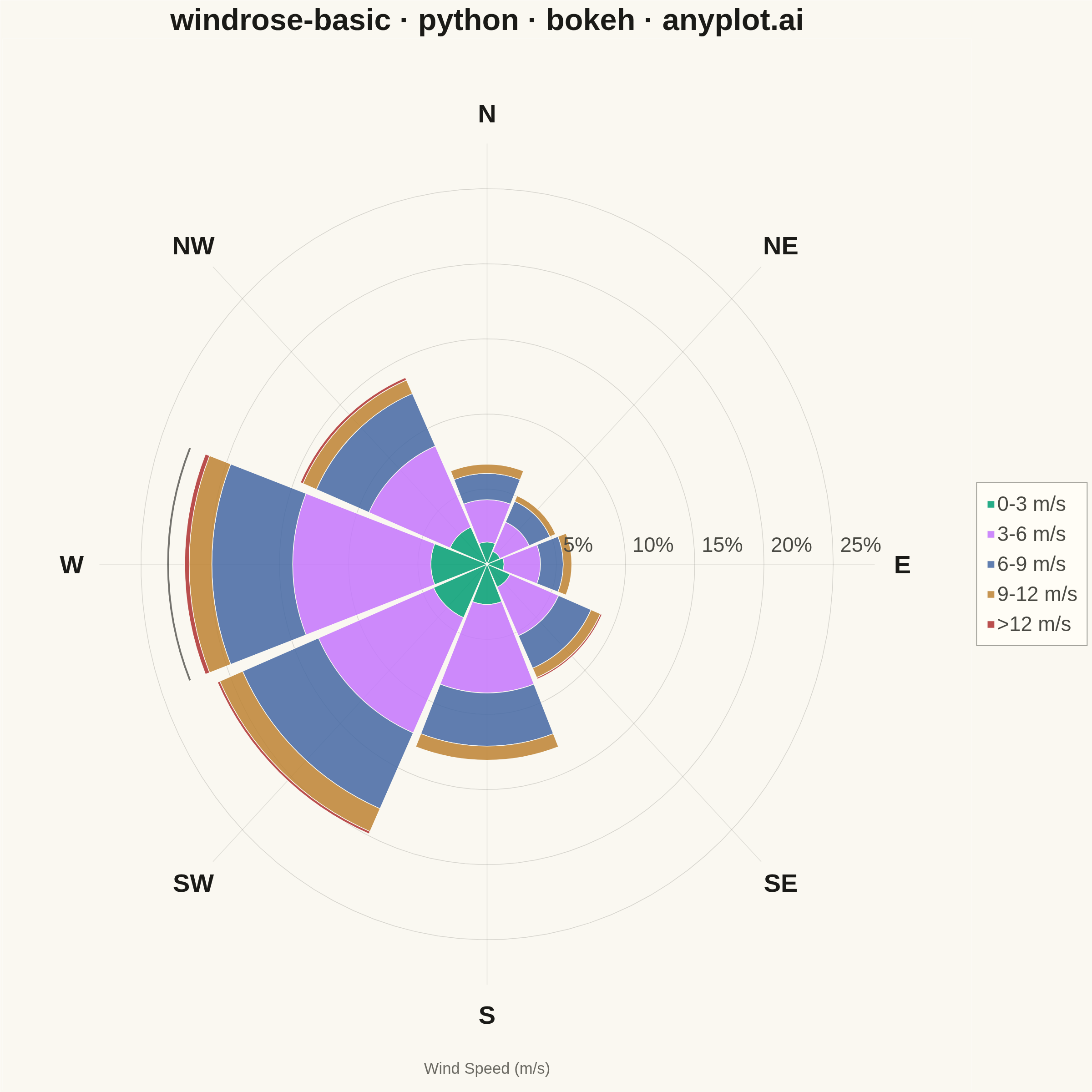
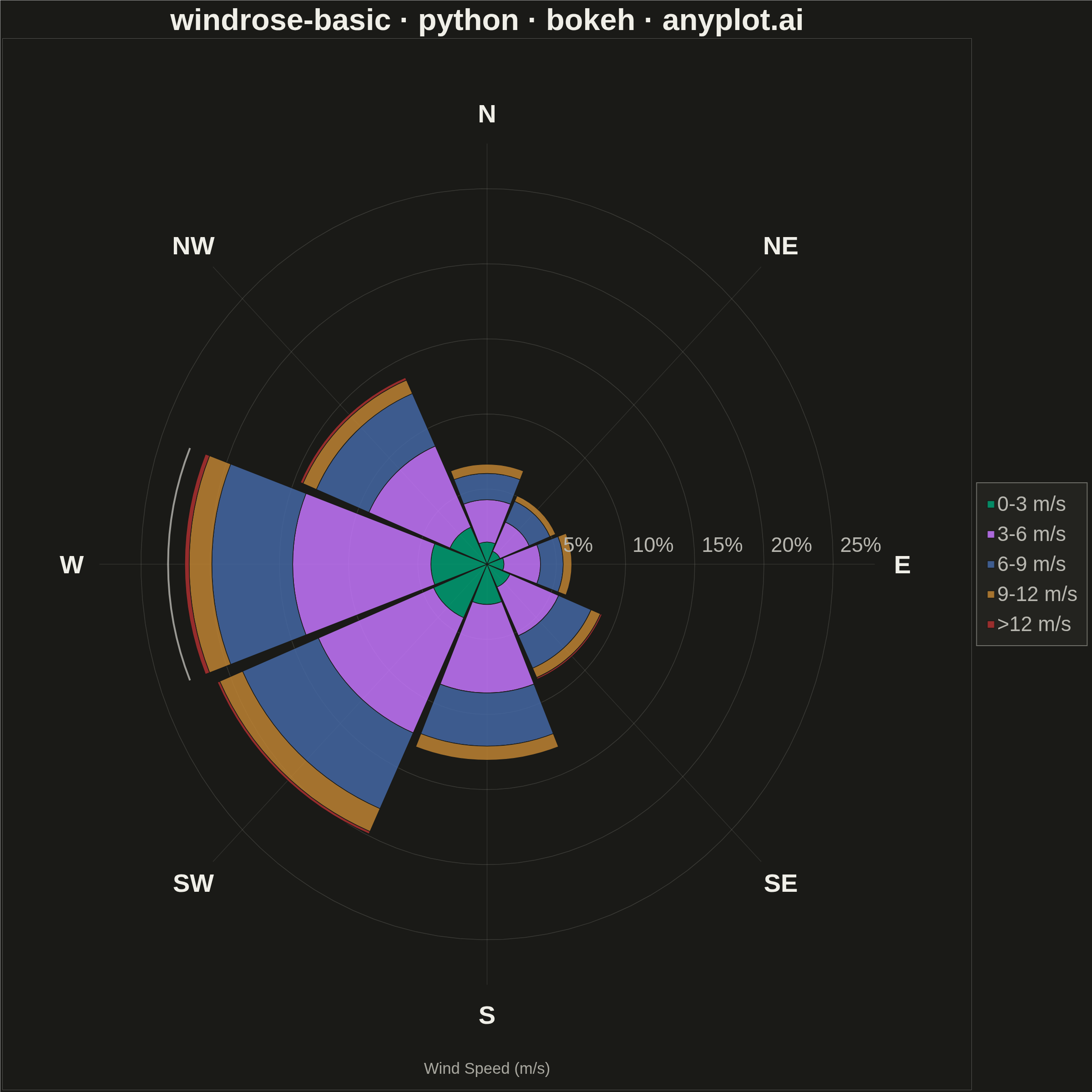
A wind rose displays wind speed and direction data as a polar stacked histogram showing the frequency distribution of wind across compass directions. Each spoke represents a direction sector (typically 8-16 bins), with stacked colored segments indicating different wind speed ranges. This specialized meteorological visualization reveals dominant wind patterns, prevailing directions, and speed distributions simultaneously, making it essential for site assessment and environmental analysis.
""" anyplot.ai
windrose-basic: Wind Rose Chart
Library: bokeh 3.9.2 | Python 3.13.14
Quality: 94/100 | Updated: 2026-08-05
"""

import os
import time
from pathlib import Path

import numpy as np
from bokeh.io import output_file, save
from bokeh.models import ColumnDataSource, Legend, LegendItem
from bokeh.plotting import figure
from selenium import webdriver
from selenium.webdriver.chrome.options import Options


# Theme tokens
THEME = os.getenv("ANYPLOT_THEME", "light")
PAGE_BG = "#FAF8F1" if THEME == "light" else "#1A1A17"
ELEVATED_BG = "#FFFDF6" if THEME == "light" else "#242420"
INK = "#1A1A17" if THEME == "light" else "#F0EFE8"
INK_SOFT = "#4A4A44" if THEME == "light" else "#B8B7B0"
INK_MUTED = "#6B6A63" if THEME == "light" else "#A8A79F"

# Imprint palette (canonical order) for speed bins, low to high
IMPRINT = ["#009E73", "#C475FD", "#4467A3", "#BD8233", "#AE3030"]

# Data - Generate realistic wind data for a coastal weather station
np.random.seed(42)
n_observations = 5000

# Direction distribution favoring SW and W winds (common for coastal areas)
direction_weights = [0.08, 0.06, 0.05, 0.08, 0.10, 0.18, 0.25, 0.20]  # N, NE, E, SE, S, SW, W, NW
directions_idx = np.random.choice(8, size=n_observations, p=direction_weights)
direction_noise = np.random.uniform(-22.5, 22.5, n_observations)
directions = directions_idx * 45 + direction_noise
directions = directions % 360

# Wind speed with Weibull distribution (realistic for wind data)
speeds = np.random.weibull(2.2, n_observations) * 6  # Scale for m/s

# Define bins
direction_bins = np.linspace(0, 360, 9)  # 8 direction sectors
direction_labels = ["N", "NE", "E", "SE", "S", "SW", "W", "NW"]
speed_bins = [0, 3, 6, 9, 12, np.inf]  # m/s ranges
speed_labels = ["0-3 m/s", "3-6 m/s", "6-9 m/s", "9-12 m/s", ">12 m/s"]

# Aggregate data into direction/speed bins
dir_indices = np.digitize(directions, direction_bins) - 1
dir_indices = np.clip(dir_indices, 0, 7)
speed_indices = np.digitize(speeds, speed_bins) - 1
speed_indices = np.clip(speed_indices, 0, len(speed_bins) - 2)

# Calculate frequencies for each direction/speed combination
frequencies = np.zeros((8, len(speed_bins) - 1))
for d_idx in range(8):
    for s_idx in range(len(speed_bins) - 1):
        frequencies[d_idx, s_idx] = np.sum((dir_indices == d_idx) & (speed_indices == s_idx))

# Convert to percentages
frequencies = frequencies / n_observations * 100

# Create figure - square format for polar-like display
p = figure(
    width=2400,
    height=2400,
    title="windrose-basic · python · bokeh · anyplot.ai",
    x_range=(-35, 35),
    y_range=(-35, 35),
    match_aspect=True,  # keep wedges/circles round even though the legend eats frame width
    tools="",
    toolbar_location=None,
)

# Style title and overall appearance
p.title.text_font_size = "50pt"
p.title.text_color = INK
p.title.align = "center"

# Theme-adaptive background
p.background_fill_color = PAGE_BG
p.border_fill_color = PAGE_BG
p.outline_line_color = None

# Hide axes for polar plot
p.xaxis.visible = False
p.yaxis.visible = False
p.xgrid.visible = False
p.ygrid.visible = False

# Draw concentric circles for reference (grid sits below the data)
sector_width = 2 * np.pi / 8  # 45 degrees in radians
for radius in [5, 10, 15, 20, 25]:
    theta_circle = np.linspace(0, 2 * np.pi, 100)
    x_circle = radius * np.cos(theta_circle)
    y_circle = radius * np.sin(theta_circle)
    p.line(x_circle, y_circle, line_color=INK_SOFT, line_width=1.5, line_alpha=0.2)

# Draw direction spokes (grid sits below the data)
for i in range(8):
    angle = np.pi / 2 - i * sector_width  # Start from North (top), go clockwise
    x_spoke = [0, 28 * np.cos(angle)]
    y_spoke = [0, 28 * np.sin(angle)]
    p.line(x_spoke, y_spoke, line_color=INK_SOFT, line_width=1.5, line_alpha=0.15)

# Stack each direction's speed bins from the center outward
center_angles = np.pi / 2 - np.arange(8) * sector_width  # North = up, clockwise
inner_radii = np.zeros((8, len(speed_labels)))
outer_radii = np.zeros((8, len(speed_labels)))
cumulative = np.zeros(8)
for speed_idx in range(len(speed_labels)):
    inner_radii[:, speed_idx] = cumulative
    cumulative = cumulative + frequencies[:, speed_idx]
    outer_radii[:, speed_idx] = cumulative
total_freq = cumulative  # total stacked height per direction

# Draw each speed bin as one vectorized annular_wedge glyph (bokeh's native
# polar/radial primitive) spanning all 8 directions, instead of hand-built
# polygons — a single ColumnDataSource + glyph call per bin.
legend_items = []
gap = 0.02  # radians of separation between neighboring direction sectors
for speed_idx in range(len(speed_labels)):
    mask = frequencies[:, speed_idx] > 0.1  # only draw significant bins
    if not mask.any():
        continue
    source = ColumnDataSource(
        data={
            "inner_radius": inner_radii[mask, speed_idx],
            "outer_radius": outer_radii[mask, speed_idx],
            "start_angle": center_angles[mask] - sector_width / 2 + gap,
            "end_angle": center_angles[mask] + sector_width / 2 - gap,
        }
    )
    renderer = p.annular_wedge(
        x=0,
        y=0,
        inner_radius="inner_radius",
        outer_radius="outer_radius",
        start_angle="start_angle",
        end_angle="end_angle",
        source=source,
        fill_color=IMPRINT[speed_idx],
        fill_alpha=0.85,
        line_color=PAGE_BG,
        line_width=1.5,
    )
    legend_items.append(LegendItem(label=speed_labels[speed_idx], renderers=[renderer]))

# Highlight the dominant direction with a thin accent ring just outside its
# stack — a deliberate emphasis technique beyond the data's natural sizing.
dominant_idx = int(np.argmax(total_freq))
dominant_angle = center_angles[dominant_idx]
p.arc(
    x=0,
    y=0,
    radius=total_freq[dominant_idx] + 1.2,
    start_angle=dominant_angle - sector_width / 2 + gap,
    end_angle=dominant_angle + sector_width / 2 - gap,
    line_color=INK,
    line_width=4,
    line_alpha=0.6,
)

# Frequency and direction labels are added last so they render on top of the
# wedges — added earlier, bokeh's default draw order let the wedges paint over
# the grid text wherever a sector's stacked height reached that far outward.
for radius in [5, 10, 15, 20, 25]:
    p.text(
        x=[radius + 0.5],
        y=[0.5],
        text=[f"{radius}%"],
        text_font_size="34pt",
        text_color=INK_SOFT,
        text_baseline="bottom",
    )

for i, label in enumerate(direction_labels):
    angle = np.pi / 2 - i * sector_width  # Start from North (top), go clockwise
    label_radius = 30
    x_label = label_radius * np.cos(angle)
    y_label = label_radius * np.sin(angle)
    p.text(
        x=[x_label],
        y=[y_label],
        text=[label],
        text_font_size="42pt",
        text_font_style="bold",
        text_color=INK,
        text_align="center",
        text_baseline="middle",
    )

# Add legend with theme-adaptive styling
legend = Legend(
    items=legend_items,
    location="center",
    label_text_font_size="34pt",
    label_text_color=INK_SOFT,
    spacing=14,
    padding=20,
    background_fill_alpha=0.95,
    background_fill_color=ELEVATED_BG,
    border_line_color=INK_SOFT,
    border_line_width=2,
)
p.add_layout(legend, "right")

# Add subtitle with data info
p.text(
    x=[0],
    y=[-33],
    text=["Wind Speed (m/s)"],
    text_font_size="26pt",
    text_color=INK_MUTED,
    text_align="center",
    text_baseline="top",
)

# Save as HTML
output_file(f"plot-{THEME}.html")
save(p)

# Screenshot with headless Chrome — Selenium 4 / Selenium Manager auto-resolves a working driver
W, H = 2400, 2400
opts = Options()
for arg in (
    "--headless=new",
    "--no-sandbox",
    "--disable-dev-shm-usage",
    "--disable-gpu",
    f"--window-size={W},{H}",
    "--hide-scrollbars",
):
    opts.add_argument(arg)
driver = webdriver.Chrome(options=opts)
driver.set_window_size(W, H)
driver.get(f"file://{Path(f'plot-{THEME}.html').resolve()}")
# headless Chrome's --window-size sets the OUTER window, which still reserves a
# phantom title-bar height even headless — pin the viewport exactly via CDP.
driver.execute_cdp_cmd(
    "Emulation.setDeviceMetricsOverride", {"width": W, "height": H, "deviceScaleFactor": 1, "mobile": False}
)
time.sleep(3)  # let bokeh's JS render the canvas
driver.save_screenshot(f"plot-{THEME}.png")
driver.quit()
Runnable source as JSON, for any HTTP client: https://api.anyplot.ai/specs/windrose-basic/bokeh/code. Any spec id and library id listed in llms-full.txt fit the same URL shape; every URL below is complete and callable.
{
  "spec_id": "windrose-basic",
  "language": "python",
  "library": "bokeh",
  "page": "https://anyplot.ai/windrose-basic/python/bokeh",
  "hub": "https://anyplot.ai/windrose-basic",
  "code_json": "https://api.anyplot.ai/specs/windrose-basic/bokeh/code",
  "spec_json": "https://api.anyplot.ai/specs/windrose-basic",
  "render_light_png": "https://storage.googleapis.com/anyplot-images/plots/windrose-basic/python/bokeh/plot-light.png",
  "render_dark_png": "https://storage.googleapis.com/anyplot-images/plots/windrose-basic/python/bokeh/plot-dark.png",
  "interactive_light_html": "https://storage.googleapis.com/anyplot-images/plots/windrose-basic/python/bokeh/plot-light.html",
  "interactive_dark_html": "https://storage.googleapis.com/anyplot-images/plots/windrose-basic/python/bokeh/plot-dark.html",
  "quality_score": 94.0,
  "license": "MIT",
  "guide": "https://anyplot.ai/llms.txt"
}
Part of Wind Rose Chart on anyplot.ai.