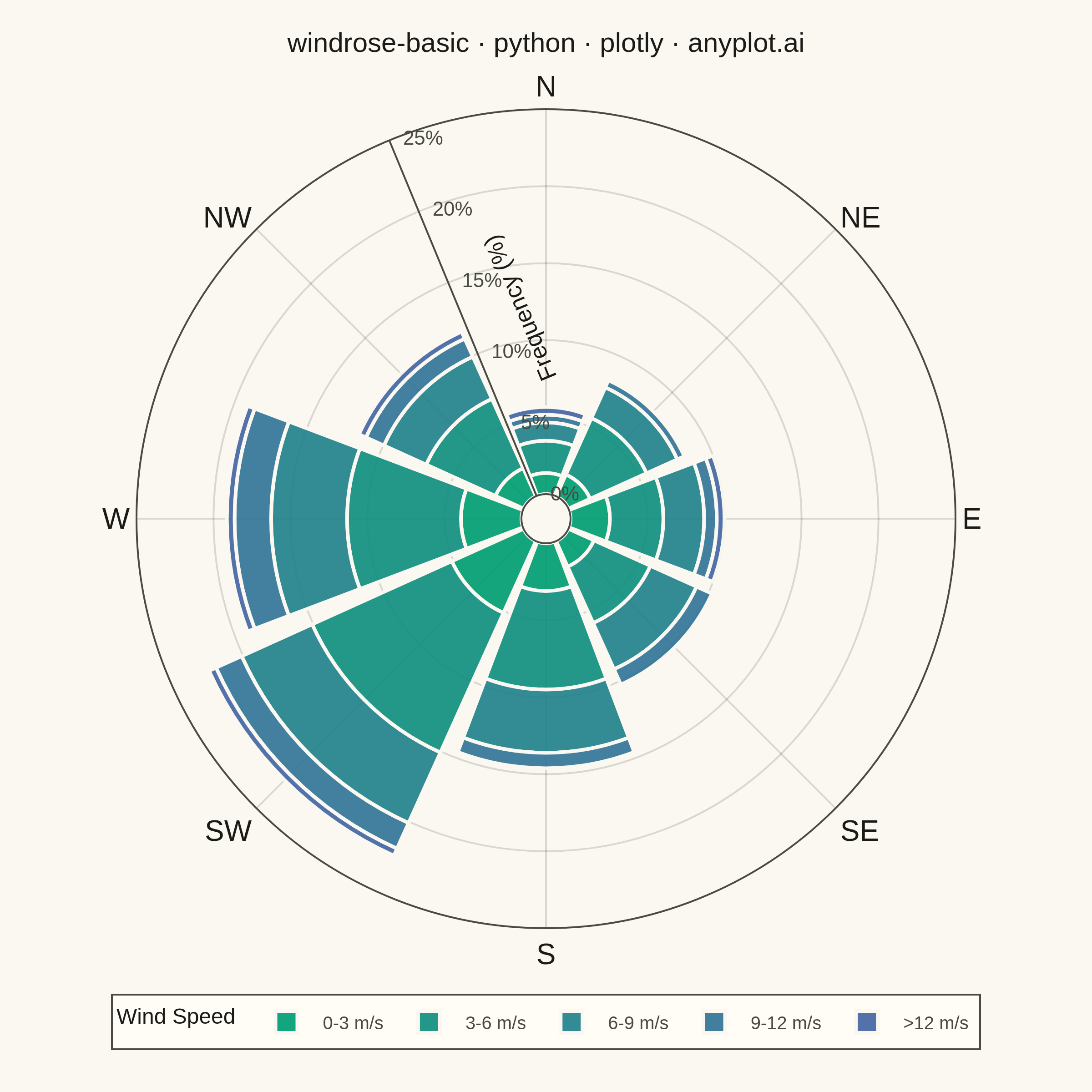
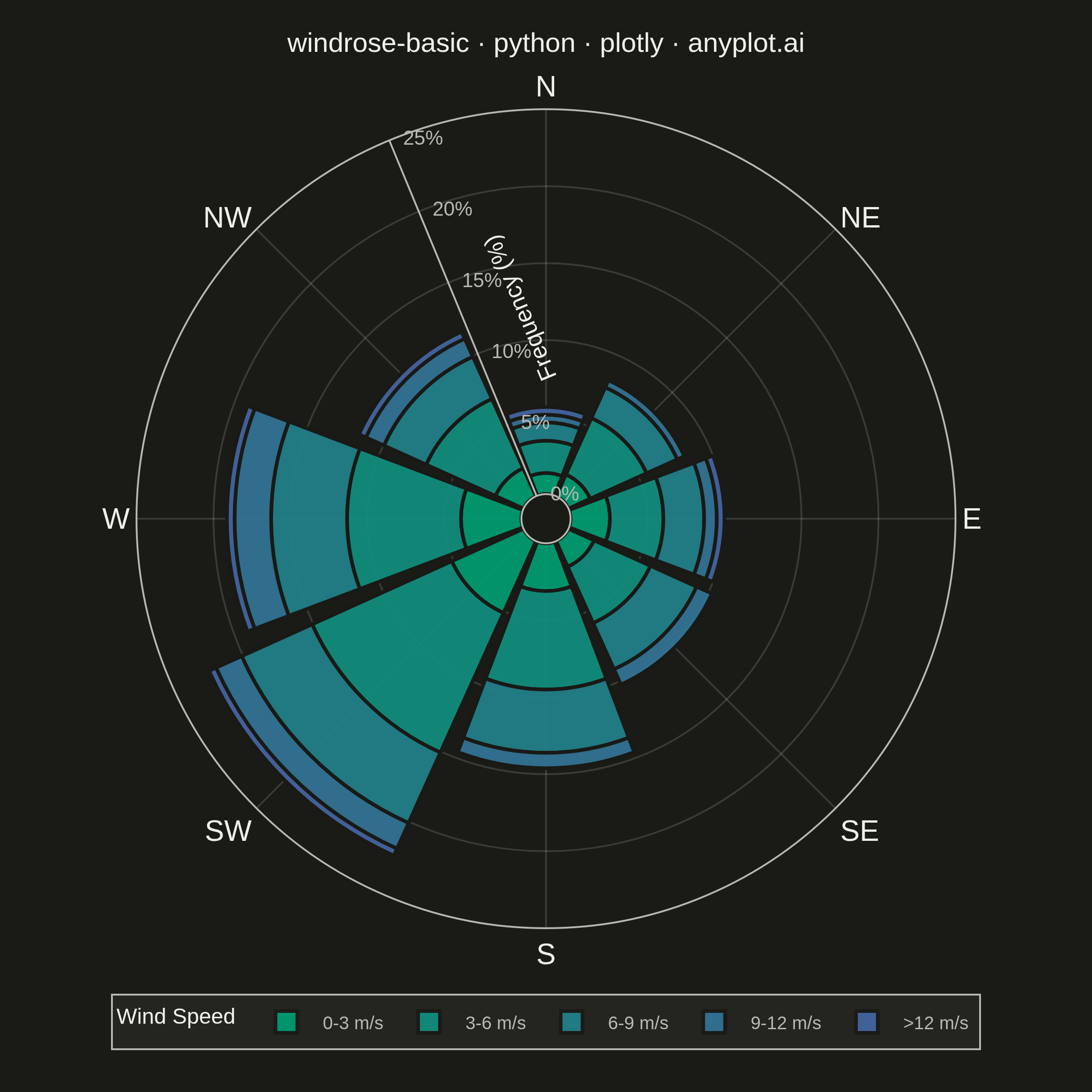
A wind rose displays wind speed and direction data as a polar stacked histogram showing the frequency distribution of wind across compass directions. Each spoke represents a direction sector (typically 8-16 bins), with stacked colored segments indicating different wind speed ranges. This specialized meteorological visualization reveals dominant wind patterns, prevailing directions, and speed distributions simultaneously, making it essential for site assessment and environmental analysis.
""" anyplot.ai
windrose-basic: Wind Rose Chart
Library: plotly 6.9.0 | Python 3.13.14
Quality: 90/100 | Updated: 2026-08-05
"""

import os

import numpy as np
import plotly.graph_objects as go
from plotly.colors import sample_colorscale


# Theme tokens
THEME = os.getenv("ANYPLOT_THEME", "light")
PAGE_BG = "#FAF8F1" if THEME == "light" else "#1A1A17"
ELEVATED_BG = "#FFFDF6" if THEME == "light" else "#242420"
INK = "#1A1A17" if THEME == "light" else "#F0EFE8"
INK_SOFT = "#4A4A44" if THEME == "light" else "#B8B7B0"
GRID = "rgba(26,26,23,0.15)" if THEME == "light" else "rgba(240,239,232,0.15)"

# Data - Daily-average wind measurements from a coastal monitoring mast, 3-year record
# (long-term climatology, distinct from a single hourly-observation year)
np.random.seed(42)
n_observations = 1095  # 3 years of daily readings

# Simulate wind direction with prevailing westerly and southwesterly winds
direction_weights = np.array([0.05, 0.05, 0.08, 0.10, 0.12, 0.20, 0.25, 0.15])  # N, NE, E, SE, S, SW, W, NW
directions_base = np.array([0, 45, 90, 135, 180, 225, 270, 315])
direction_idx = np.random.choice(8, size=n_observations, p=direction_weights)
directions = directions_base[direction_idx] + np.random.uniform(-20, 20, n_observations)
directions = directions % 360

# Simulate wind speeds with realistic distribution (Weibull-like)
speeds = np.random.weibull(2.0, n_observations) * 6  # Scale for realistic m/s values

# Define direction bins (8 sectors, 45 degrees each)
dir_bins = np.array([0, 45, 90, 135, 180, 225, 270, 315, 360])
dir_labels = ["N", "NE", "E", "SE", "S", "SW", "W", "NW"]

# Define speed bins (m/s) - ordinal magnitude, so colored with the Imprint sequential
# colormap (imprint_seq: brand green -> blue) rather than the categorical palette
speed_bins = [0, 3, 6, 9, 12, np.inf]
speed_labels = ["0-3 m/s", "3-6 m/s", "6-9 m/s", "9-12 m/s", ">12 m/s"]
imprint_seq = [[0.0, "#009E73"], [1.0, "#4467A3"]]
speed_colors = sample_colorscale(imprint_seq, [i / (len(speed_labels) - 1) for i in range(len(speed_labels))])

# Bin the data
dir_indices = np.digitize(directions, dir_bins[:-1]) - 1
dir_indices = np.clip(dir_indices, 0, 7)
speed_indices = np.digitize(speeds, speed_bins[:-1]) - 1

# Calculate frequencies for each direction and speed combination
frequencies = np.zeros((8, 5))
for d in range(8):
    for s in range(5):
        frequencies[d, s] = np.sum((dir_indices == d) & (speed_indices == s))

# Convert to percentages
frequencies_pct = frequencies / n_observations * 100

# Keep the rarest speed tier perceptible even at sub-1% frequency
frequencies_pct = np.where((frequencies_pct > 0) & (frequencies_pct < 0.5), 0.5, frequencies_pct)

# Create wind rose using barpolar
fig = go.Figure()

# Add traces for each speed bin (stacked from inside to outside)
for s in range(5):
    r_values = frequencies_pct[:, s]

    fig.add_trace(
        go.Barpolar(
            r=r_values,
            theta=dir_labels,
            name=speed_labels[s],
            marker_color=speed_colors[s],
            marker_line_color=PAGE_BG,
            marker_line_width=2,
            opacity=0.92,
            hovertemplate=f"<b>%{{theta}}</b><br>{speed_labels[s]}: %{{r:.1f}}%<extra></extra>",
        )
    )

# Update layout for proper stacking and styling
fig.update_layout(
    autosize=False,
    width=600,
    height=600,
    title={
        "text": "windrose-basic · python · plotly · anyplot.ai",
        "font": {"size": 15, "color": INK},
        "x": 0.5,
        "xanchor": "center",
        "y": 0.97,
    },
    paper_bgcolor=PAGE_BG,
    plot_bgcolor=PAGE_BG,
    font={"color": INK},
    polar={
        "hole": 0.06,
        "bargap": 0.08,
        "radialaxis": {
            "visible": True,
            "showticklabels": True,
            "tickfont": {"size": 11, "color": INK_SOFT},
            "ticksuffix": "%",
            "angle": 112.5,
            "tickangle": 112.5,
            "dtick": 5,
            "range": [0, 25],
            "title": {"text": "Frequency (%)", "font": {"size": 13, "color": INK}},
            "gridcolor": GRID,
            "linecolor": INK_SOFT,
        },
        "angularaxis": {
            "tickfont": {"size": 16, "color": INK},
            "direction": "clockwise",
            "rotation": 90,
            "categoryorder": "array",
            "categoryarray": ["N", "NE", "E", "SE", "S", "SW", "W", "NW"],
            "gridcolor": GRID,
            "linecolor": INK_SOFT,
        },
        "bgcolor": PAGE_BG,
    },
    legend={
        "title": {"text": "Wind Speed", "font": {"size": 12, "color": INK}},
        "font": {"size": 10, "color": INK_SOFT},
        "x": 0.5,
        "y": -0.08,
        "xanchor": "center",
        "yanchor": "top",
        "orientation": "h",
        "bgcolor": ELEVATED_BG,
        "bordercolor": INK_SOFT,
        "borderwidth": 1,
    },
    barmode="stack",
    margin={"l": 40, "r": 40, "t": 60, "b": 90},
)

# Save as PNG and HTML
fig.write_image(f"plot-{THEME}.png", width=600, height=600, scale=4)
fig.write_html(f"plot-{THEME}.html", include_plotlyjs="cdn")
Runnable source as JSON, for any HTTP client: https://api.anyplot.ai/specs/windrose-basic/plotly/code. Any spec id and library id listed in llms-full.txt fit the same URL shape; every URL below is complete and callable.
{
  "spec_id": "windrose-basic",
  "language": "python",
  "library": "plotly",
  "page": "https://anyplot.ai/windrose-basic/python/plotly",
  "hub": "https://anyplot.ai/windrose-basic",
  "code_json": "https://api.anyplot.ai/specs/windrose-basic/plotly/code",
  "spec_json": "https://api.anyplot.ai/specs/windrose-basic",
  "render_light_png": "https://storage.googleapis.com/anyplot-images/plots/windrose-basic/python/plotly/plot-light.png",
  "render_dark_png": "https://storage.googleapis.com/anyplot-images/plots/windrose-basic/python/plotly/plot-dark.png",
  "interactive_light_html": "https://storage.googleapis.com/anyplot-images/plots/windrose-basic/python/plotly/plot-light.html",
  "interactive_dark_html": "https://storage.googleapis.com/anyplot-images/plots/windrose-basic/python/plotly/plot-dark.html",
  "quality_score": 90.0,
  "license": "MIT",
  "guide": "https://anyplot.ai/llms.txt"
}
Part of Wind Rose Chart on anyplot.ai.