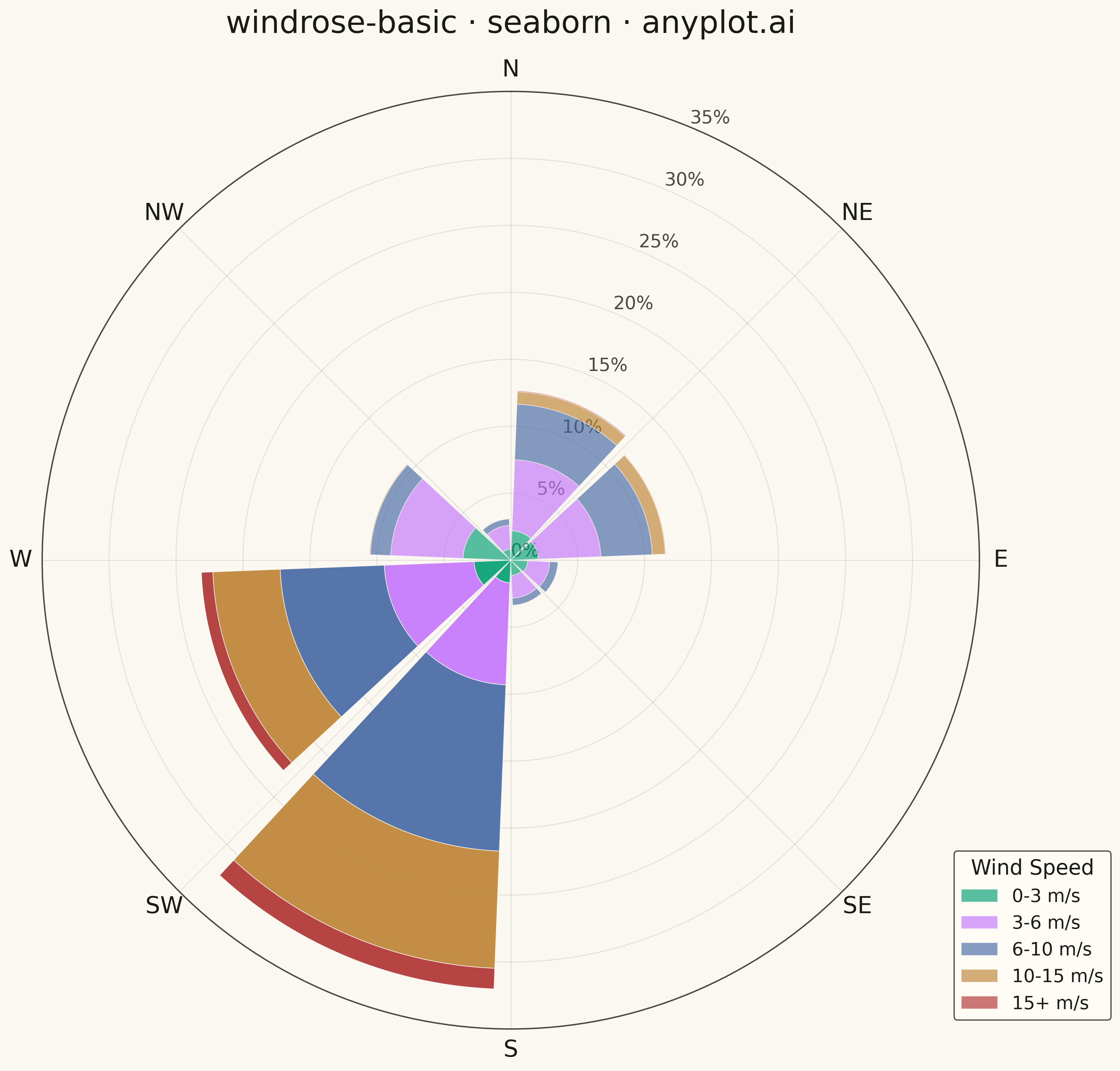
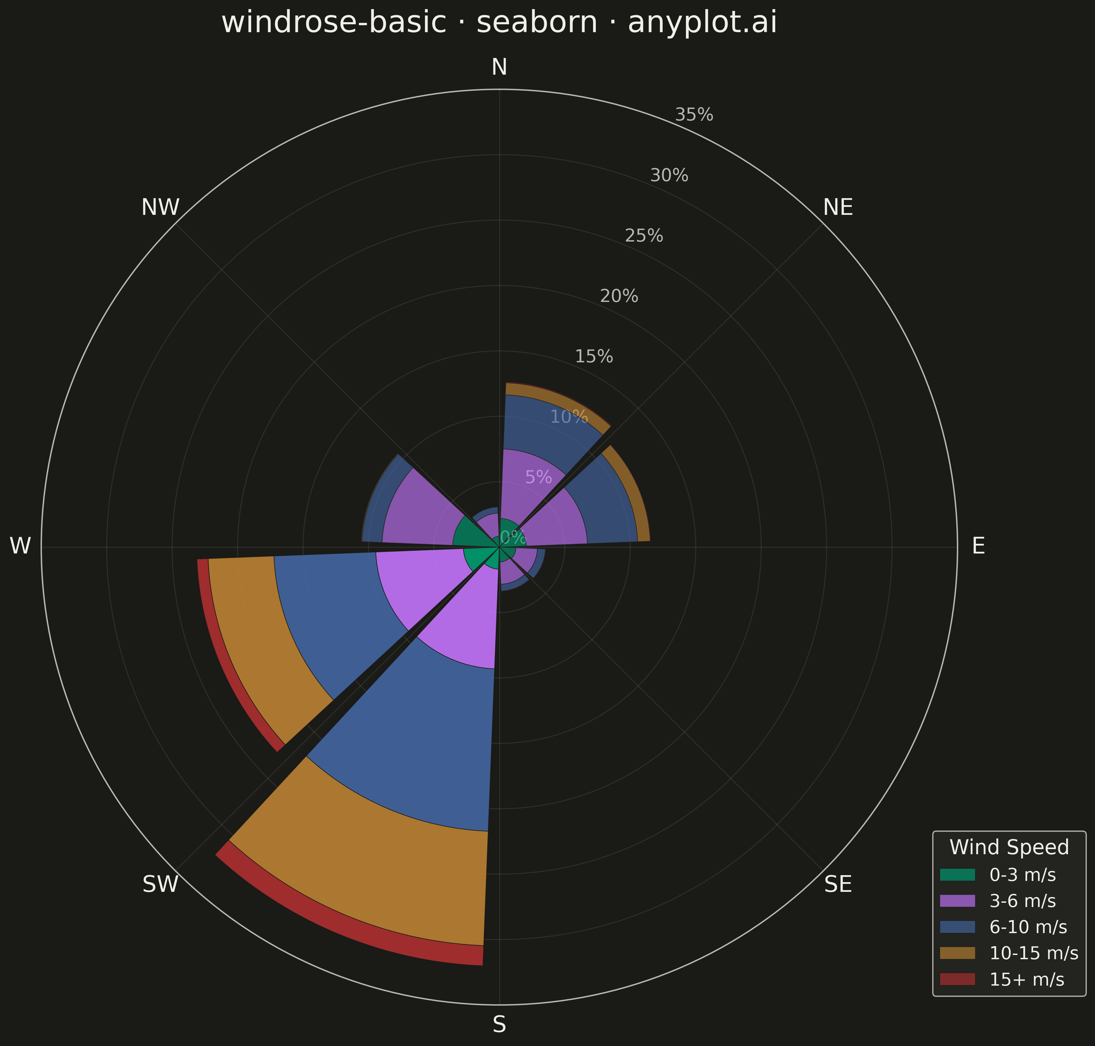
A wind rose displays wind speed and direction data as a polar stacked histogram showing the frequency distribution of wind across compass directions. Each spoke represents a direction sector (typically 8-16 bins), with stacked colored segments indicating different wind speed ranges. This specialized meteorological visualization reveals dominant wind patterns, prevailing directions, and speed distributions simultaneously, making it essential for site assessment and environmental analysis.
""" anyplot.ai
windrose-basic: Wind Rose Chart
Library: seaborn 0.13.2 | Python 3.13.13
Quality: 88/100 | Updated: 2026-05-07
"""

import os

import matplotlib.pyplot as plt
import numpy as np
import seaborn as sns


# Theme tokens
THEME = os.getenv("ANYPLOT_THEME", "light")
PAGE_BG = "#FAF8F1" if THEME == "light" else "#1A1A17"
ELEVATED_BG = "#FFFDF6" if THEME == "light" else "#242420"
INK = "#1A1A17" if THEME == "light" else "#F0EFE8"
INK_SOFT = "#4A4A44" if THEME == "light" else "#B8B7B0"

# Okabe-Ito palette for speed ranges (cool to warm progression)
IMPRINT = ["#009E73", "#C475FD", "#4467A3", "#BD8233", "#AE3030"]

# Configure seaborn
sns.set_theme(
    style="ticks",
    rc={
        "figure.facecolor": PAGE_BG,
        "axes.facecolor": PAGE_BG,
        "axes.labelcolor": INK,
        "text.color": INK,
        "xtick.color": INK_SOFT,
        "ytick.color": INK_SOFT,
        "grid.color": INK_SOFT,
        "grid.alpha": 0.10,
        "legend.facecolor": ELEVATED_BG,
        "legend.edgecolor": INK_SOFT,
    },
)

# Data
np.random.seed(42)
n_obs = 8760

# Simulate prevailing winds with realistic distribution
direction_weights = np.zeros(360)
direction_weights[200:240] = 3.0
direction_weights[30:60] = 1.5
direction_weights[260:290] = 1.0
direction_weights += 0.2
direction_weights /= direction_weights.sum()

directions = np.random.choice(360, size=n_obs, p=direction_weights)
directions = (directions + np.random.uniform(-10, 10, n_obs)) % 360

# Wind speeds by direction
speeds = np.zeros(n_obs)
for i, d in enumerate(directions):
    if 200 <= d <= 240:
        speeds[i] = np.random.weibull(2.2) * 8 + 2
    elif 30 <= d <= 60:
        speeds[i] = np.random.weibull(2.0) * 6 + 1
    else:
        speeds[i] = np.random.weibull(1.8) * 4 + 0.5
speeds = np.clip(speeds, 0, 25)

# 8-direction bins (N, NE, E, SE, S, SW, W, NW)
n_dir_bins = 8
dir_bins = np.linspace(0, 360, n_dir_bins + 1)
dir_centers = (dir_bins[:-1] + dir_bins[1:]) / 2
dir_width = 2 * np.pi / n_dir_bins

# Speed bins
speed_bins = [0, 3, 6, 10, 15, 25]
speed_labels = ["0-3 m/s", "3-6 m/s", "6-10 m/s", "10-15 m/s", "15+ m/s"]

# Calculate frequencies
frequencies = np.zeros((n_dir_bins, len(speed_labels)))
for i in range(n_dir_bins):
    dir_min, dir_max = dir_bins[i], dir_bins[i + 1]
    in_dir = (directions >= dir_min) & (directions < dir_max)

    for j in range(len(speed_labels)):
        speed_min = speed_bins[j]
        speed_max = speed_bins[j + 1]
        in_speed = (speeds >= speed_min) & (speeds < speed_max)
        frequencies[i, j] = np.sum(in_dir & in_speed)

frequencies = frequencies / n_obs * 100

# Plot
fig = plt.figure(figsize=(12, 12), facecolor=PAGE_BG)
ax = fig.add_subplot(111, projection="polar")

ax.set_facecolor(PAGE_BG)
ax.set_theta_zero_location("N")
ax.set_theta_direction(-1)

theta = np.deg2rad(dir_centers)

# Identify prevailing wind sectors (highest frequency) for visual emphasis
total_freq = frequencies.sum(axis=1)
dominant_threshold = np.percentile(total_freq, 75)
is_dominant = total_freq > dominant_threshold

# Plot stacked bars with Okabe-Ito palette
bottoms = np.zeros(n_dir_bins)
for j, (label, color) in enumerate(zip(speed_labels, IMPRINT, strict=False)):
    # Use full alpha for dominant sectors, reduced for weaker ones
    alpha_per_sector = np.where(is_dominant, 0.90, 0.65)

    # Plot all sectors in one call, then manually adjust alpha if possible
    bars = ax.bar(
        theta,
        frequencies[:, j],
        width=dir_width * 0.9,
        bottom=bottoms,
        color=color,
        edgecolor=PAGE_BG,
        linewidth=0.5,
        label=label,
        alpha=0.85,
    )

    # Adjust individual bar alpha for dominant directions
    for bar, alpha_val in zip(bars, alpha_per_sector, strict=False):
        bar.set_alpha(alpha_val)

    bottoms += frequencies[:, j]

# Style
ax.set_title("windrose-basic · seaborn · anyplot.ai", fontsize=24, pad=20, fontweight="medium", color=INK)

max_freq = np.ceil(bottoms.max() / 5) * 5
ax.set_ylim(0, max_freq)
ax.set_yticks(np.arange(0, max_freq + 1, 5))
ax.set_yticklabels([f"{int(y)}%" for y in np.arange(0, max_freq + 1, 5)], fontsize=14, color=INK_SOFT)

direction_labels = ["N", "NE", "E", "SE", "S", "SW", "W", "NW"]
ax.set_xticks(np.deg2rad(np.arange(0, 360, 45)))
ax.set_xticklabels(direction_labels, fontsize=18, fontweight="medium", color=INK)

# Enhanced grid styling with subtle radial emphasis
ax.grid(True, alpha=0.12, linestyle="-", linewidth=0.8, color=INK_SOFT)
for spine in ax.spines.values():
    spine.set_color(INK_SOFT)
    spine.set_linewidth(1.1)

legend = ax.legend(
    title="Wind Speed", loc="lower right", bbox_to_anchor=(1.15, 0), fontsize=14, title_fontsize=16, framealpha=0.95
)
legend.get_frame().set_facecolor(ELEVATED_BG)
legend.get_frame().set_edgecolor(INK_SOFT)
legend.get_title().set_color(INK)
for text in legend.get_texts():
    text.set_color(INK)

plt.tight_layout()
plt.savefig(f"plot-{THEME}.png", dpi=300, bbox_inches="tight", facecolor=PAGE_BG)
Runnable source as JSON, for any HTTP client: https://api.anyplot.ai/specs/windrose-basic/seaborn/code. Any spec id and library id listed in llms-full.txt fit the same URL shape; every URL below is complete and callable.
{
  "spec_id": "windrose-basic",
  "language": "python",
  "library": "seaborn",
  "page": "https://anyplot.ai/windrose-basic/python/seaborn",
  "hub": "https://anyplot.ai/windrose-basic",
  "code_json": "https://api.anyplot.ai/specs/windrose-basic/seaborn/code",
  "spec_json": "https://api.anyplot.ai/specs/windrose-basic",
  "render_light_png": "https://storage.googleapis.com/anyplot-images/plots/windrose-basic/python/seaborn/plot-light.png",
  "render_dark_png": "https://storage.googleapis.com/anyplot-images/plots/windrose-basic/python/seaborn/plot-dark.png",
  "quality_score": 88.0,
  "license": "MIT",
  "guide": "https://anyplot.ai/llms.txt"
}
Part of Wind Rose Chart on anyplot.ai.