The same plot in 14 other libraries — Python: Altair, Bokeh, lets-plot, Matplotlib, Plotly, plotnine, Pygal, Seaborn; Julia: Makie.jl; JavaScript: Chart.js, D3.js, Apache ECharts, Highcharts, MUI X Charts. Compare all 15 side by side: Basic 3D Wireframe Plot in Python, R, Julia and JavaScript.
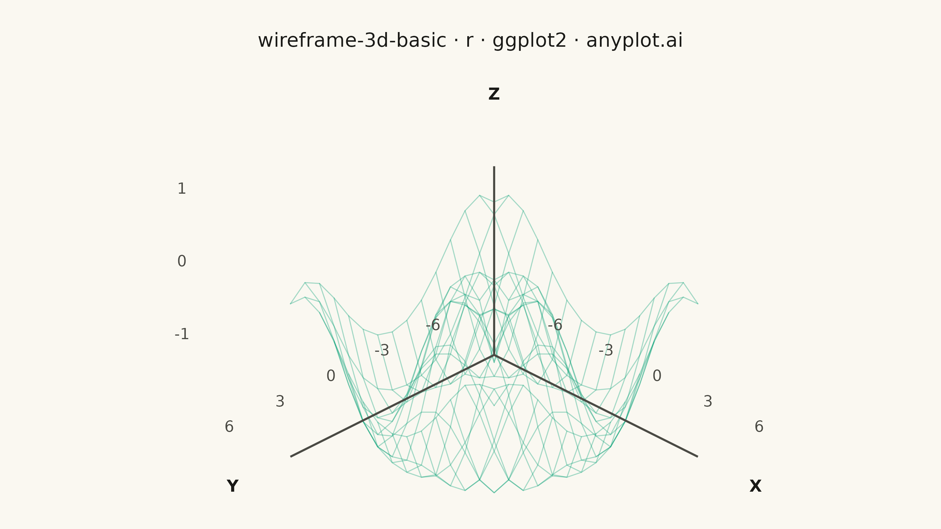
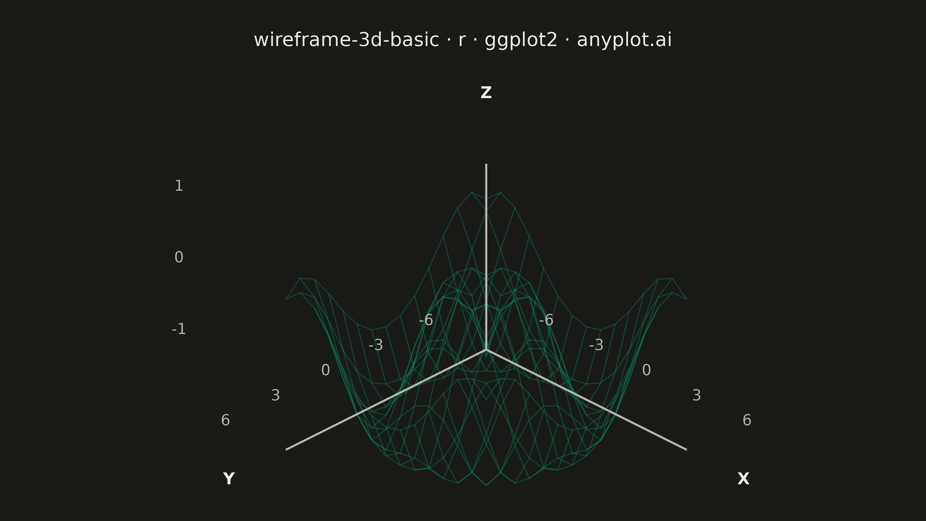
A 3D wireframe plot displays a mathematical surface as a mesh of lines connecting grid points in three-dimensional space. Unlike solid surface plots, wireframes render only the edges between grid points, creating a see-through visualization that reveals the underlying structure and allows viewing parts of the surface that would otherwise be hidden. This makes wireframes ideal for understanding the topology and shape of 3D functions.
#' anyplot.ai
#' wireframe-3d-basic: Basic 3D Wireframe Plot
#' Library: ggplot2 3.5.1 | R 4.4.1
#' Quality: 87/100 | Updated: 2026-09-10

library(ggplot2)
library(ragg)

set.seed(42)

# --- Theme tokens -------------------------------------------------------------
THEME    <- Sys.getenv("ANYPLOT_THEME", "light")
PAGE_BG  <- if (THEME == "light") "#FAF8F1" else "#1A1A17"
INK      <- if (THEME == "light") "#1A1A17" else "#F0EFE8"
INK_SOFT <- if (THEME == "light") "#4A4A44" else "#B8B7B0"
BRAND    <- "#009E73"

# --- Camera: orthographic projection (elevation 30, azimuth 45) ---------------
# ggplot2 has no 3D grammar, so the mesh is projected to 2D screen coordinates
# ourselves (the same technique any static 3D renderer uses under the hood),
# then drawn with plain geom_polygon/geom_segment/geom_text.
elev <- 30 * pi / 180
azim <- 45 * pi / 180

view_dir  <- c(cos(elev) * cos(azim), cos(elev) * sin(azim), sin(elev))
world_up  <- c(0, 0, 1)
right_axis <- c(
  view_dir[2] * world_up[3] - view_dir[3] * world_up[2],
  view_dir[3] * world_up[1] - view_dir[1] * world_up[3],
  view_dir[1] * world_up[2] - view_dir[2] * world_up[1]
)
right_axis <- right_axis / sqrt(sum(right_axis^2))
up_axis <- c(
  right_axis[2] * view_dir[3] - right_axis[3] * view_dir[2],
  right_axis[3] * view_dir[1] - right_axis[1] * view_dir[3],
  right_axis[1] * view_dir[2] - right_axis[2] * view_dir[1]
)

z_lift <- 3.5  # visual height exaggeration so the shallow ripple reads clearly
project_x <- function(x, y, z) x * right_axis[1] + y * right_axis[2] + z * z_lift * right_axis[3]
project_y <- function(x, y, z) x * up_axis[1]    + y * up_axis[2]    + z * z_lift * up_axis[3]
depth_toward_camera <- function(x, y, z) x * view_dir[1] + y * view_dir[2] + z * z_lift * view_dir[3]

# --- Data: ripple surface z = sin(sqrt(x^2 + y^2)) -----------------------------
grid_n <- 30
x_vals <- seq(-6, 6, length.out = grid_n)
y_vals <- seq(-6, 6, length.out = grid_n)
z_fun  <- function(x, y) sin(sqrt(x^2 + y^2))

z_range <- range(outer(x_vals, y_vals, z_fun))
floor_z <- z_range[1] - 0.3
ceil_z  <- z_range[2] + 0.3

# --- Mesh quads with painter's-algorithm hidden-line removal ------------------
# Each grid cell becomes a filled quad. Quads are drawn back-to-front (farthest
# from the camera first) with an opaque page-background fill, so nearer quads
# occlude the grid lines sitting behind them - the same trick base R's persp()
# uses instead of a real z-buffer. This lets the mesh resolution sit inside the
# spec's recommended 20x20-50x50 range without the interior crosshatching a
# flat semi-transparent wireframe produces.
n_cells <- (grid_n - 1)^2
mesh <- data.frame(
  quad_id = integer(n_cells * 4),
  corner  = integer(n_cells * 4),
  px      = numeric(n_cells * 4),
  py      = numeric(n_cells * 4)
)
quad_depth <- numeric(n_cells)

row  <- 1
quad <- 1
for (i in seq_len(grid_n - 1)) {
  for (j in seq_len(grid_n - 1)) {
    cx <- c(x_vals[i], x_vals[i + 1], x_vals[i + 1], x_vals[i])
    cy <- c(y_vals[j], y_vals[j],     y_vals[j + 1],  y_vals[j + 1])
    cz <- z_fun(cx, cy)
    idx <- row:(row + 3)
    mesh$quad_id[idx] <- quad
    mesh$corner[idx]  <- 1:4
    mesh$px[idx] <- project_x(cx, cy, cz)
    mesh$py[idx] <- project_y(cx, cy, cz)
    quad_depth[quad] <- mean(depth_toward_camera(cx, cy, cz))
    row  <- row + 4
    quad <- quad + 1
  }
}

# Farthest quad gets draw_rank 1 (painted first); nearest gets n_cells (painted
# last, on top). The fill itself must stay fully opaque for the occlusion to
# work - only the edge colour's alpha channel is faded with depth, as a subtle
# depth cue (bolder edges up close, softer far away).
draw_rank      <- rank(quad_depth, ties.method = "first")
mesh$draw_rank <- draw_rank[mesh$quad_id]
fade           <- 0.55 + 0.45 * (mesh$draw_rank - 1) / (n_cells - 1)
brand_rgb      <- col2rgb(BRAND) / 255
mesh$edge_color <- rgb(brand_rgb[1], brand_rgb[2], brand_rgb[3], alpha = fade)
mesh <- mesh[order(mesh$draw_rank, mesh$corner), ]

# --- Floor reference plane (spatial grounding) ---------------------------------
floor_plane <- data.frame(
  x = c(-6, 6, 6, -6),
  y = c(-6, -6, 6, 6),
  z = floor_z
)
floor_plane$px <- project_x(floor_plane$x, floor_plane$y, floor_plane$z)
floor_plane$py <- project_y(floor_plane$x, floor_plane$y, floor_plane$z)

# --- Axis box: three edges meeting at the front-left-bottom corner ------------
axis_lines <- data.frame(
  x    = c(-6, -6, -6),
  y    = c(-6, -6, -6),
  z    = c(floor_z, floor_z, floor_z),
  xend = c(6, -6, -6),
  yend = c(-6, 6, -6),
  zend = c(floor_z, floor_z, ceil_z)
)
axis_lines$px    <- project_x(axis_lines$x, axis_lines$y, axis_lines$z)
axis_lines$py    <- project_y(axis_lines$x, axis_lines$y, axis_lines$z)
axis_lines$pxend <- project_x(axis_lines$xend, axis_lines$yend, axis_lines$zend)
axis_lines$pyend <- project_y(axis_lines$xend, axis_lines$yend, axis_lines$zend)

x_breaks <- c(-6, -3, 0, 3, 6)
y_breaks <- c(-6, -3, 0, 3, 6)
z_breaks <- c(-1, 0, 1)

ticks <- rbind(
  data.frame(x = x_breaks, y = -9.6, z = floor_z, label = x_breaks, axis = "x"),
  data.frame(x = -9.6, y = y_breaks, z = floor_z, label = y_breaks, axis = "y")
)
ticks$px <- project_x(ticks$x, ticks$y, ticks$z)
ticks$py <- project_y(ticks$x, ticks$y, ticks$z)

# The X-tick and Y-tick label columns sit on the mesh's near side, where the
# wireframe's screen footprint is widest, so a couple of low-value ticks
# ("-3"/"-6") land inside the mesh's silhouette instead of clearing it. Nudge
# each column sideways, away from the vertical Z axis, by a fixed screen
# offset (same lateral-offset trick used for z_ticks below) - harmless for
# the ticks that already clear the mesh, since it just adds margin.
tick_clearance <- 5.5
ticks$px <- ticks$px + ifelse(ticks$axis == "x", tick_clearance, -tick_clearance)

# Z ticks sit on the vertical axis line itself; nudge the label text
# (not the axis line) sideways into the open gap left of the mesh, well past
# the Y-axis tick column so the two label groups don't merge into one line.
z_ticks <- data.frame(x = -6, y = -6, z = z_breaks, label = z_breaks)
z_ticks$px <- project_x(z_ticks$x, z_ticks$y, z_ticks$z) - 13
z_ticks$py <- project_y(z_ticks$x, z_ticks$y, z_ticks$z)

axis_labels <- data.frame(
  x     = c(9.4, -6, -6),
  y     = c(-6, 9.4, -6),
  z     = c(floor_z, floor_z, ceil_z + 1.0),
  label = c("X", "Y", "Z")
)
axis_labels$px <- project_x(axis_labels$x, axis_labels$y, axis_labels$z)
axis_labels$py <- project_y(axis_labels$x, axis_labels$y, axis_labels$z)

# --- Plot -----------------------------------------------------------------
p <- ggplot() +
  geom_polygon(data = floor_plane, aes(px, py),
               fill = NA, color = INK_SOFT, linewidth = 0.4, alpha = 0.4) +
  geom_polygon(data = mesh, aes(px, py, group = draw_rank, colour = I(edge_color)),
               fill = PAGE_BG, linewidth = 0.25) +
  geom_segment(data = axis_lines, aes(x = px, y = py, xend = pxend, yend = pyend),
               color = INK_SOFT, linewidth = 0.6) +
  geom_text(data = ticks, aes(px, py, label = label),
            color = INK_SOFT, size = 3.3) +
  geom_text(data = z_ticks, aes(px, py, label = label),
            color = INK_SOFT, size = 3.3) +
  geom_text(data = axis_labels, aes(px, py, label = label),
            color = INK, size = 3.6, fontface = "bold") +
  labs(title = "wireframe-3d-basic · r · ggplot2 · anyplot.ai") +
  coord_fixed(ratio = 1, clip = "off") +
  theme_void(base_size = 8) +
  theme(
    plot.background  = element_rect(fill = PAGE_BG, color = PAGE_BG),
    panel.background = element_rect(fill = PAGE_BG, color = NA),
    plot.title       = element_text(color = INK, size = 12, hjust = 0.5, margin = margin(b = 14)),
    plot.margin      = margin(t = 20, r = 30, b = 10, l = 30)
  )

# --- Save -----------------------------------------------------------------
ggsave(
  filename = sprintf("plot-%s.png", THEME),
  plot     = p,
  device   = ragg::agg_png,
  width    = 8,
  height   = 4.5,
  units    = "in",
  dpi      = 400
)
Runnable source as JSON, for any HTTP client: https://api.anyplot.ai/specs/wireframe-3d-basic/ggplot2/code. Any spec id and library id listed in llms-full.txt fit the same URL shape; every URL below is complete and callable.
{
  "spec_id": "wireframe-3d-basic",
  "language": "r",
  "library": "ggplot2",
  "page": "https://anyplot.ai/wireframe-3d-basic/r/ggplot2",
  "hub": "https://anyplot.ai/wireframe-3d-basic",
  "code_json": "https://api.anyplot.ai/specs/wireframe-3d-basic/ggplot2/code",
  "spec_json": "https://api.anyplot.ai/specs/wireframe-3d-basic",
  "render_light_png": "https://storage.googleapis.com/anyplot-images/plots/wireframe-3d-basic/r/ggplot2/plot-light.png",
  "render_dark_png": "https://storage.googleapis.com/anyplot-images/plots/wireframe-3d-basic/r/ggplot2/plot-dark.png",
  "quality_score": 87.0,
  "license": "MIT",
  "guide": "https://anyplot.ai/llms.txt"
}
Part of Basic 3D Wireframe Plot on anyplot.ai.