The same plot in 14 other libraries — Python: Altair, Bokeh, lets-plot, Matplotlib, Plotly, plotnine, Pygal, Seaborn; Julia: Makie.jl; JavaScript: Chart.js, D3.js, Apache ECharts, Highcharts, MUI X Charts. Compare all 15 side by side: Basic Heatmap in Python, R, Julia and JavaScript.
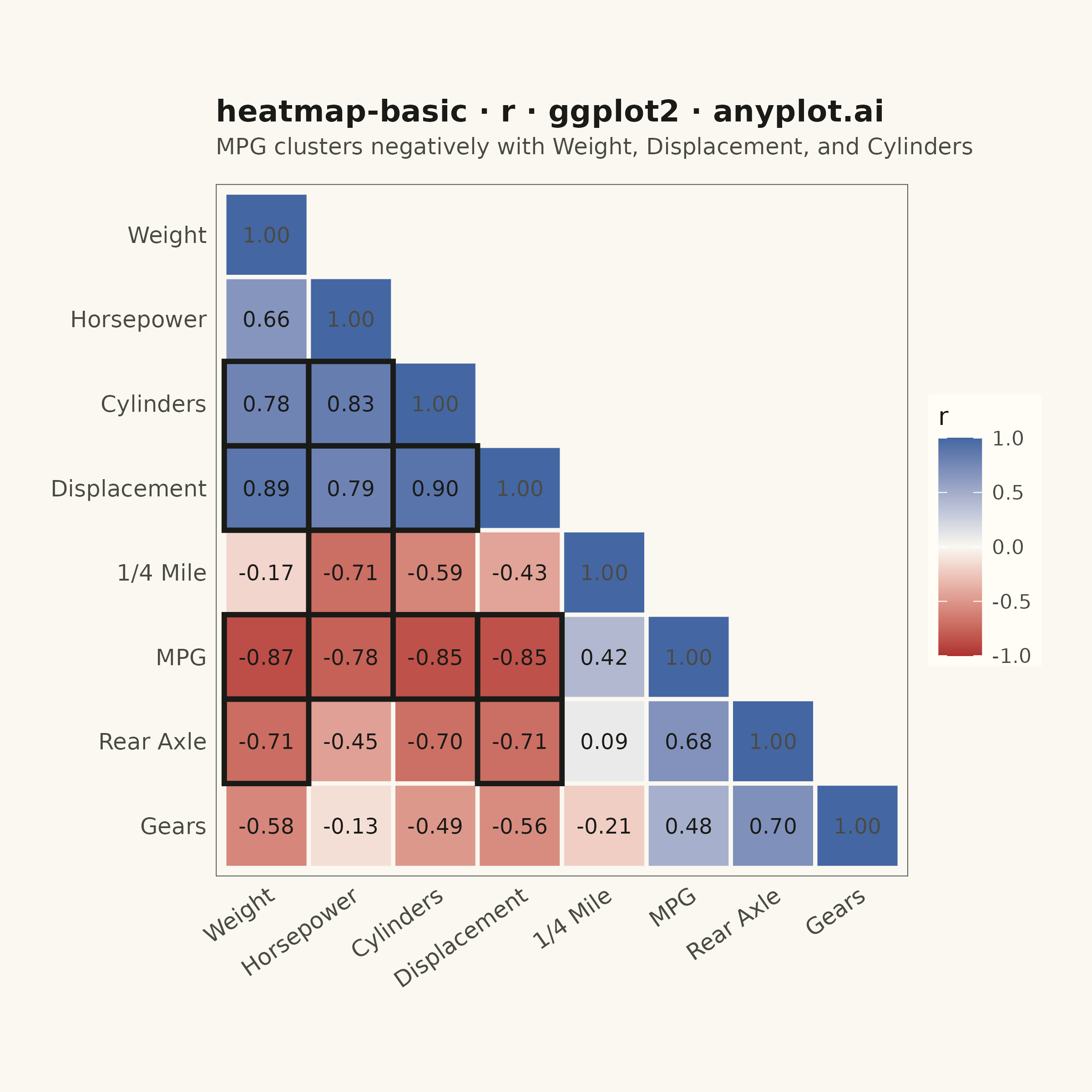
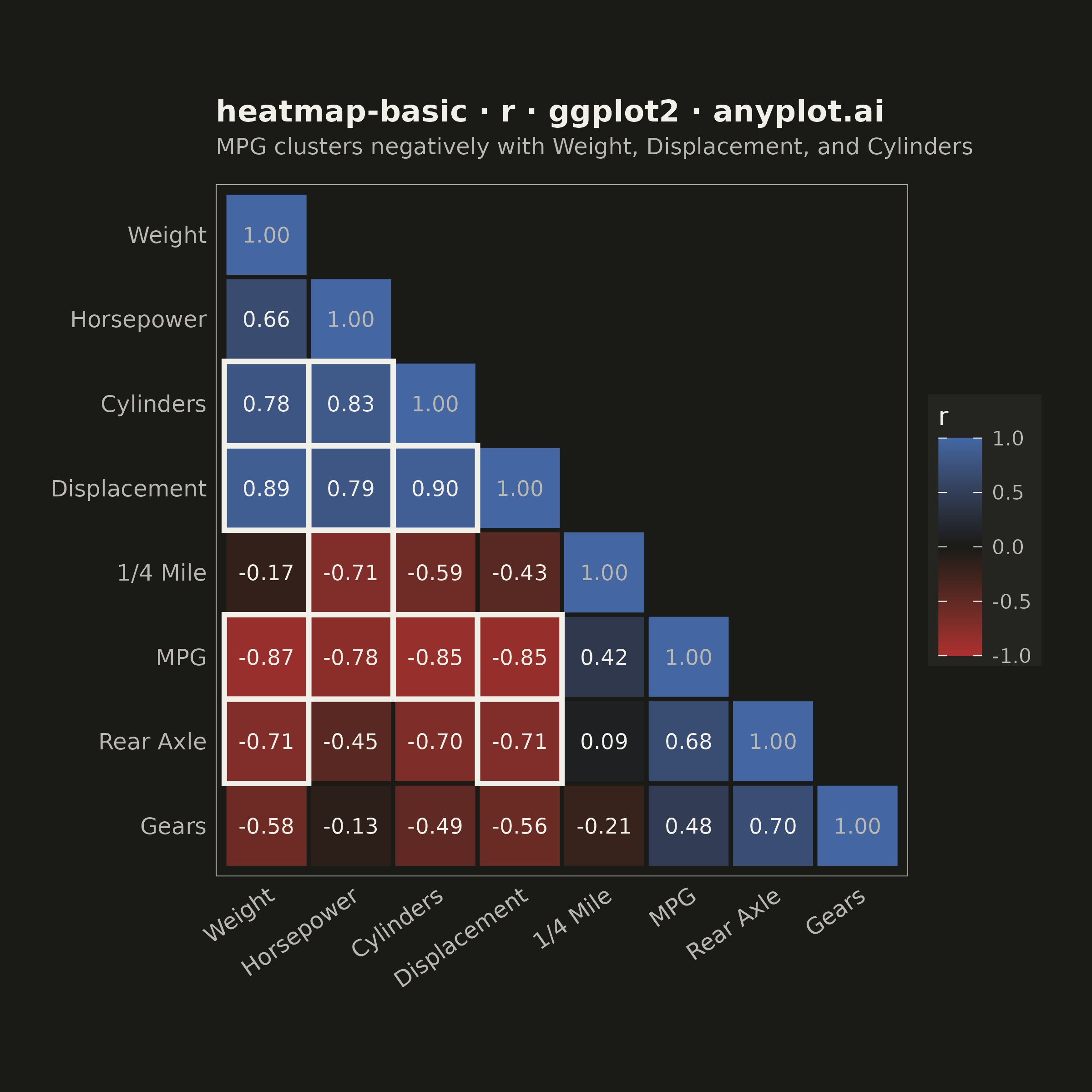
A heatmap displaying values in a matrix format using color intensity. Each cell's color represents the magnitude of the value, making it easy to identify patterns, clusters, and outliers in two-dimensional data. Essential for visualizing correlations, frequencies, and relationships between variables.
#' anyplot.ai
#' heatmap-basic: Basic Heatmap
#' Library: ggplot2 3.5.1 | R 4.4.1
#' Quality: 91/100 | Created: 2026-05-28

library(ggplot2)
library(tidyr)
library(ragg)

# Theme tokens
THEME       <- Sys.getenv("ANYPLOT_THEME", "light")
PAGE_BG     <- if (THEME == "light") "#FAF8F1" else "#1A1A17"
ELEVATED_BG <- if (THEME == "light") "#FFFDF6" else "#242420"
INK         <- if (THEME == "light") "#1A1A17" else "#F0EFE8"
INK_SOFT    <- if (THEME == "light") "#4A4A44" else "#B8B7B0"
DIV_MID     <- if (THEME == "light") "#FAF8F1" else "#1A1A17"

# Data: pairwise correlations across mtcars vehicle performance metrics
data(mtcars)
selected_vars <- c("mpg", "cyl", "disp", "hp", "drat", "wt", "qsec", "gear")
var_labels    <- c("MPG", "Cylinders", "Displacement", "Horsepower",
                   "Rear Axle", "Weight", "1/4 Mile", "Gears")

cor_mat           <- cor(mtcars[, selected_vars])
rownames(cor_mat) <- var_labels
colnames(cor_mat) <- var_labels

# Reorder variables by hierarchical clustering — groups similar variables together
hc_order  <- hclust(as.dist(1 - cor_mat))$order
hc_labels <- var_labels[hc_order]

# Reshape to long format
cor_df       <- as.data.frame(cor_mat)
cor_df$y_var <- rownames(cor_df)
cor_long     <- pivot_longer(cor_df, cols = -y_var,
                             names_to = "x_var", values_to = "correlation")

# Lower triangle masking (including diagonal) to eliminate redundancy
x_idx    <- match(cor_long$x_var, hc_labels)
y_idx    <- match(cor_long$y_var, hc_labels)
cor_long <- cor_long[y_idx >= x_idx, ]

# Apply clustered ordering; reverse y levels so diagonal runs top-left to bottom-right
cor_long$x_var <- factor(cor_long$x_var, levels = hc_labels)
cor_long$y_var <- factor(cor_long$y_var, levels = rev(hc_labels))

# Mark diagonal cells and strong off-diagonal correlations for visual treatment
cor_long$on_diag   <- as.character(cor_long$x_var) == as.character(cor_long$y_var)
cor_long$is_strong <- abs(cor_long$correlation) > 0.7 & !cor_long$on_diag

plot_title    <- "heatmap-basic · r · ggplot2 · anyplot.ai"
plot_subtitle <- "MPG clusters negatively with Weight, Displacement, and Cylinders"

p <- ggplot(cor_long, aes(x = x_var, y = y_var, fill = correlation)) +
  geom_tile(color = PAGE_BG, linewidth = 0.8) +
  # Highlight border on strong off-diagonal correlations (|r| > 0.7)
  geom_tile(data = cor_long[cor_long$is_strong, ],
            fill = NA, color = INK, linewidth = 1.0) +
  # Off-diagonal annotations in INK; diagonal (trivial 1.00) in INK_SOFT
  geom_text(data = cor_long[!cor_long$on_diag, ],
            aes(label = sprintf("%.2f", correlation)),
            color = INK, size = 3.0) +
  geom_text(data = cor_long[cor_long$on_diag, ],
            aes(label = sprintf("%.2f", correlation)),
            color = INK_SOFT, size = 3.0) +
  scale_fill_gradient2(
    low      = "#AE3030",
    mid      = DIV_MID,
    high     = "#4467A3",
    midpoint = 0,
    limits   = c(-1, 1),
    name     = "r"
  ) +
  coord_fixed() +
  labs(title = plot_title, subtitle = plot_subtitle, x = NULL, y = NULL) +
  theme_minimal(base_size = 8) +
  theme(
    plot.background   = element_rect(fill = PAGE_BG, color = PAGE_BG),
    panel.background  = element_rect(fill = PAGE_BG, color = NA),
    panel.border      = element_rect(color = INK_SOFT, fill = NA, linewidth = 0.3),
    panel.grid        = element_blank(),
    axis.text.x       = element_text(color = INK_SOFT, size = 9,
                                     angle = 35, hjust = 1),
    axis.text.y       = element_text(color = INK_SOFT, size = 9),
    plot.title        = element_text(color = INK, size = 12, face = "bold",
                                     margin = margin(b = 4)),
    plot.subtitle     = element_text(color = INK_SOFT, size = 9,
                                     margin = margin(b = 10)),
    legend.background = element_rect(fill = ELEVATED_BG, color = NA),
    legend.text       = element_text(color = INK_SOFT, size = 8),
    legend.title      = element_text(color = INK, size = 10),
    plot.margin       = margin(20, 20, 20, 20)
  )

# Save — square canvas (2400×2400 px = 6in × 6in @ 400 dpi)
ggsave(
  filename = sprintf("plot-%s.png", THEME),
  plot     = p,
  device   = ragg::agg_png,
  width    = 6,
  height   = 6,
  units    = "in",
  dpi      = 400
)
Runnable source as JSON, for any HTTP client: https://api.anyplot.ai/specs/heatmap-basic/ggplot2/code. Any spec id and library id listed in llms-full.txt fit the same URL shape; every URL below is complete and callable.
{
  "spec_id": "heatmap-basic",
  "language": "r",
  "library": "ggplot2",
  "page": "https://anyplot.ai/heatmap-basic/r/ggplot2",
  "hub": "https://anyplot.ai/heatmap-basic",
  "code_json": "https://api.anyplot.ai/specs/heatmap-basic/ggplot2/code",
  "spec_json": "https://api.anyplot.ai/specs/heatmap-basic",
  "render_light_png": "https://storage.googleapis.com/anyplot-images/plots/heatmap-basic/r/ggplot2/plot-light.png",
  "render_dark_png": "https://storage.googleapis.com/anyplot-images/plots/heatmap-basic/r/ggplot2/plot-dark.png",
  "quality_score": 91.0,
  "license": "MIT",
  "guide": "https://anyplot.ai/llms.txt"
}
Part of Basic Heatmap on anyplot.ai.