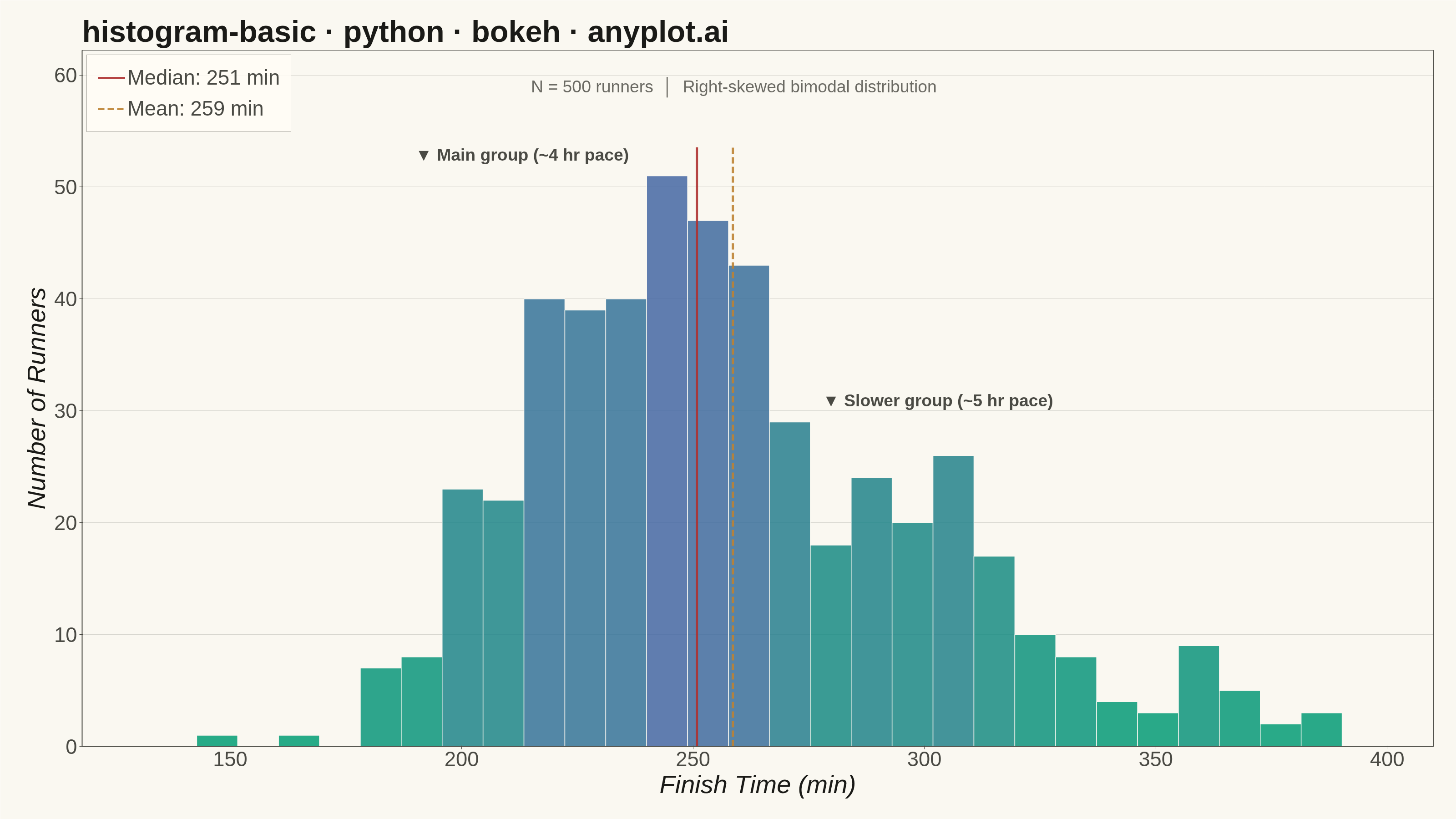
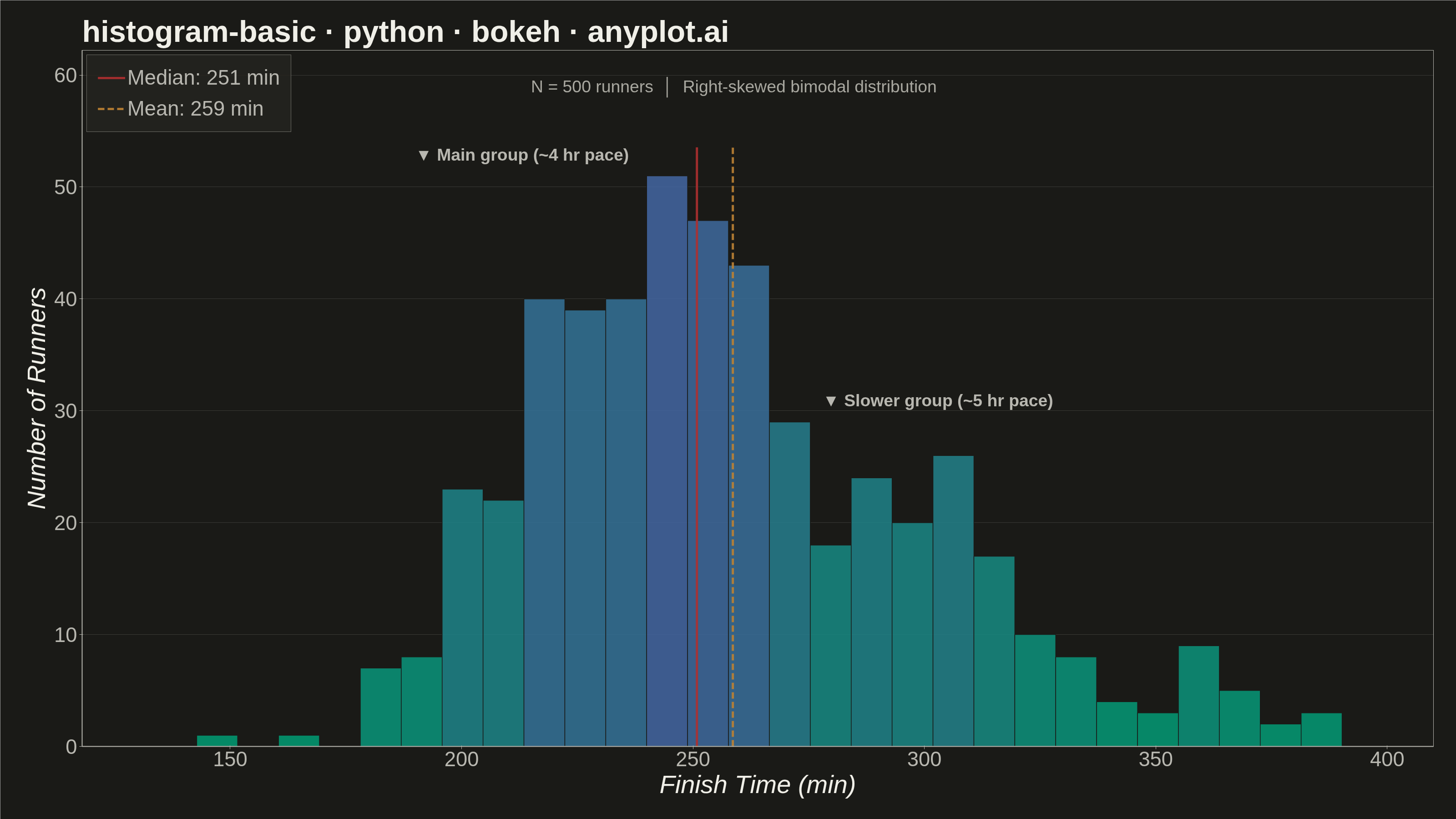
A histogram displays the distribution of a single continuous variable by dividing the data range into bins and showing the frequency (count) of observations in each bin. It reveals the shape of the data distribution, including central tendency, spread, and presence of outliers or multiple modes.
""" anyplot.ai
histogram-basic: Basic Histogram
Library: bokeh 3.9.0 | Python 3.13.13
Quality: 93/100 | Updated: 2026-05-28
"""

import io
import os
import sys
import time
from pathlib import Path

from PIL import Image


# Prevent this file's directory from shadowing the installed bokeh package
sys.path = [p for p in sys.path if os.path.abspath(p) != os.path.dirname(os.path.abspath(__file__))]

import numpy as np
from bokeh.io import output_file, save
from bokeh.models import ColumnDataSource, HoverTool, Label, Legend, LegendItem, NumeralTickFormatter
from bokeh.plotting import figure
from bokeh.transform import linear_cmap
from selenium import webdriver
from selenium.webdriver.chrome.options import Options


# Theme tokens
THEME = os.getenv("ANYPLOT_THEME", "light")
PAGE_BG = "#FAF8F1" if THEME == "light" else "#1A1A17"
ELEVATED_BG = "#FFFDF6" if THEME == "light" else "#242420"
INK = "#1A1A17" if THEME == "light" else "#F0EFE8"
INK_SOFT = "#4A4A44" if THEME == "light" else "#B8B7B0"
INK_MUTED = "#6B6A63" if THEME == "light" else "#A8A79F"

# imprint_seq colormap: brand green (#009E73) → blue (#4467A3), 256 stops
ANYPLOT_SEQ256 = [
    "#{:02X}{:02X}{:02X}".format(
        int(round(68 * t / 255)), int(round(158 - 55 * t / 255)), int(round(115 + 48 * t / 255))
    )
    for t in range(256)
]

# Data — Marathon finish times (bimodal: main recreational group + slower group)
np.random.seed(42)
main_group = np.random.normal(loc=240, scale=30, size=380)
slower_group = np.random.normal(loc=305, scale=18, size=100)
outliers = np.random.normal(loc=370, scale=12, size=20)
values = np.concatenate([main_group, slower_group, outliers])
values = values[(values > 120) & (values < 420)]

# Statistics
median_val = np.median(values)
mean_val = np.mean(values)

# Histogram bins
counts, edges = np.histogram(values, bins=28)
left_edges = edges[:-1]
right_edges = edges[1:]
max_count = int(counts.max())

source = ColumnDataSource(
    data={
        "left": left_edges,
        "right": right_edges,
        "top": counts,
        "bottom": [0] * len(counts),
        "count": counts,
        "bin_start": [f"{e:.0f}" for e in left_edges],
        "bin_end": [f"{e:.0f}" for e in right_edges],
    }
)

# imprint_seq color mapper: low count → green, high count → blue
fill_mapper = linear_cmap(field_name="top", palette=ANYPLOT_SEQ256, low=0, high=max_count)

# Figure — 3200 × 1800 px landscape
TITLE = "histogram-basic · python · bokeh · anyplot.ai"
n = len(TITLE)
title_pt = max(34, round(50 * (67 / n if n > 67 else 1.0)))
p = figure(
    width=3200,
    height=1800,
    title=TITLE,
    x_axis_label="Finish Time (min)",
    y_axis_label="Number of Runners",
    toolbar_location=None,
    x_range=(118, 410),
    min_border_bottom=160,
    min_border_left=180,
    min_border_top=110,
    min_border_right=50,
)

# Histogram bars
bars = p.quad(
    left="left",
    right="right",
    top="top",
    bottom="bottom",
    source=source,
    fill_color=fill_mapper,
    line_color=PAGE_BG,
    line_width=1.5,
    fill_alpha=0.85,
    hover_fill_color="#DDCC77",
    hover_fill_alpha=0.95,
    hover_line_color=PAGE_BG,
)

# HoverTool
hover = HoverTool(
    renderers=[bars], tooltips=[("Range", "@bin_start–@bin_end min"), ("Runners", "@count")], mode="mouse"
)
p.add_tools(hover)

# Median reference line (matte red)
median_line = p.line(
    x=[median_val, median_val], y=[0, max_count * 1.05], line_color="#AE3030", line_width=5, line_alpha=0.9
)

# Mean reference line (ochre, dashed)
mean_line = p.line(
    x=[mean_val, mean_val],
    y=[0, max_count * 1.05],
    line_color="#BD8233",
    line_width=5,
    line_dash=[14, 7],
    line_alpha=0.9,
)

# Legend — top-left, closer to the data's left shoulder
legend = Legend(
    items=[
        LegendItem(label=f"Median: {median_val:.0f} min", renderers=[median_line]),
        LegendItem(label=f"Mean: {mean_val:.0f} min", renderers=[mean_line]),
    ],
    location="top_left",
    label_text_font_size="34pt",
    label_text_color=INK_SOFT,
    glyph_width=60,
    glyph_height=6,
    spacing=16,
    padding=24,
    background_fill_color=ELEVATED_BG,
    background_fill_alpha=0.85,
    border_line_color=INK_SOFT,
    border_line_alpha=0.5,
)
p.add_layout(legend, "center")

# Annotations — main distribution peak
peak_label = Label(
    x=190,
    y=max_count * 1.02,
    text="▼ Main group (~4 hr pace)",
    text_font_size="28pt",
    text_color=INK_SOFT,
    text_font_style="bold",
)
p.add_layout(peak_label)

# Annotation — slower group shoulder
slower_peak = int(counts[np.abs(left_edges - 295) < 15].max())
shoulder_label = Label(
    x=278,
    y=slower_peak + max_count * 0.08,
    text="▼ Slower group (~5 hr pace)",
    text_font_size="28pt",
    text_color=INK_SOFT,
    text_font_style="bold",
)
p.add_layout(shoulder_label)

# Subtitle — x=215 starts right of the legend box
subtitle = Label(
    x=215,
    y=max_count * 1.14,
    text=f"N = {len(values)} runners  │  Right-skewed bimodal distribution",
    text_font_size="28pt",
    text_color=INK_MUTED,
)
p.add_layout(subtitle)

# Typography
p.title.text_font_size = f"{title_pt}pt"
p.title.text_color = INK
p.title.text_font_style = "bold"
p.xaxis.axis_label_text_font_size = "42pt"
p.yaxis.axis_label_text_font_size = "42pt"
p.xaxis.axis_label_text_color = INK
p.yaxis.axis_label_text_color = INK
p.xaxis.major_label_text_font_size = "34pt"
p.yaxis.major_label_text_font_size = "34pt"
p.xaxis.major_label_text_color = INK_SOFT
p.yaxis.major_label_text_color = INK_SOFT
p.yaxis.formatter = NumeralTickFormatter(format="0,0")

# Grid — y-axis only, very subtle
p.xgrid.visible = False
p.ygrid.grid_line_alpha = 0.15
p.ygrid.grid_line_color = INK
p.ygrid.grid_line_width = 1

# Chrome
p.outline_line_color = INK_SOFT
p.background_fill_color = PAGE_BG
p.border_fill_color = PAGE_BG
p.xaxis.axis_line_width = 2
p.yaxis.axis_line_width = 2
p.xaxis.axis_line_color = INK_SOFT
p.yaxis.axis_line_color = INK_SOFT
p.xaxis.minor_tick_line_color = None
p.yaxis.minor_tick_line_color = None
p.xaxis.major_tick_line_color = INK_SOFT
p.yaxis.major_tick_line_color = INK_SOFT
p.y_range.start = 0
p.y_range.end = max_count * 1.22

# Save HTML (interactive artifact)
output_file(f"plot-{THEME}.html")
save(p)

# Screenshot with headless Chrome — window is H+200 tall so bokeh canvas fills
# exactly W×H; PIL crops to the target rect before saving.
W, H = 3200, 1800
opts = Options()
for arg in (
    "--headless=new",
    "--no-sandbox",
    "--disable-dev-shm-usage",
    "--disable-gpu",
    f"--window-size={W},{H + 200}",
    "--hide-scrollbars",
    "--force-device-scale-factor=1",
):
    opts.add_argument(arg)
driver = webdriver.Chrome(options=opts)
driver.set_window_size(W, H + 200)
driver.get(f"file://{Path(f'plot-{THEME}.html').resolve()}")
time.sleep(3)
raw = driver.get_screenshot_as_png()
driver.quit()
Image.open(io.BytesIO(raw)).crop((0, 0, W, H)).save(f"plot-{THEME}.png")
Runnable source as JSON, for any HTTP client: https://api.anyplot.ai/specs/histogram-basic/bokeh/code. Any spec id and library id listed in llms-full.txt fit the same URL shape; every URL below is complete and callable.
{
  "spec_id": "histogram-basic",
  "language": "python",
  "library": "bokeh",
  "page": "https://anyplot.ai/histogram-basic/python/bokeh",
  "hub": "https://anyplot.ai/histogram-basic",
  "code_json": "https://api.anyplot.ai/specs/histogram-basic/bokeh/code",
  "spec_json": "https://api.anyplot.ai/specs/histogram-basic",
  "render_light_png": "https://storage.googleapis.com/anyplot-images/plots/histogram-basic/python/bokeh/plot-light.png",
  "render_dark_png": "https://storage.googleapis.com/anyplot-images/plots/histogram-basic/python/bokeh/plot-dark.png",
  "interactive_light_html": "https://storage.googleapis.com/anyplot-images/plots/histogram-basic/python/bokeh/plot-light.html",
  "interactive_dark_html": "https://storage.googleapis.com/anyplot-images/plots/histogram-basic/python/bokeh/plot-dark.html",
  "quality_score": 93.0,
  "license": "MIT",
  "guide": "https://anyplot.ai/llms.txt"
}
Part of Basic Histogram on anyplot.ai.