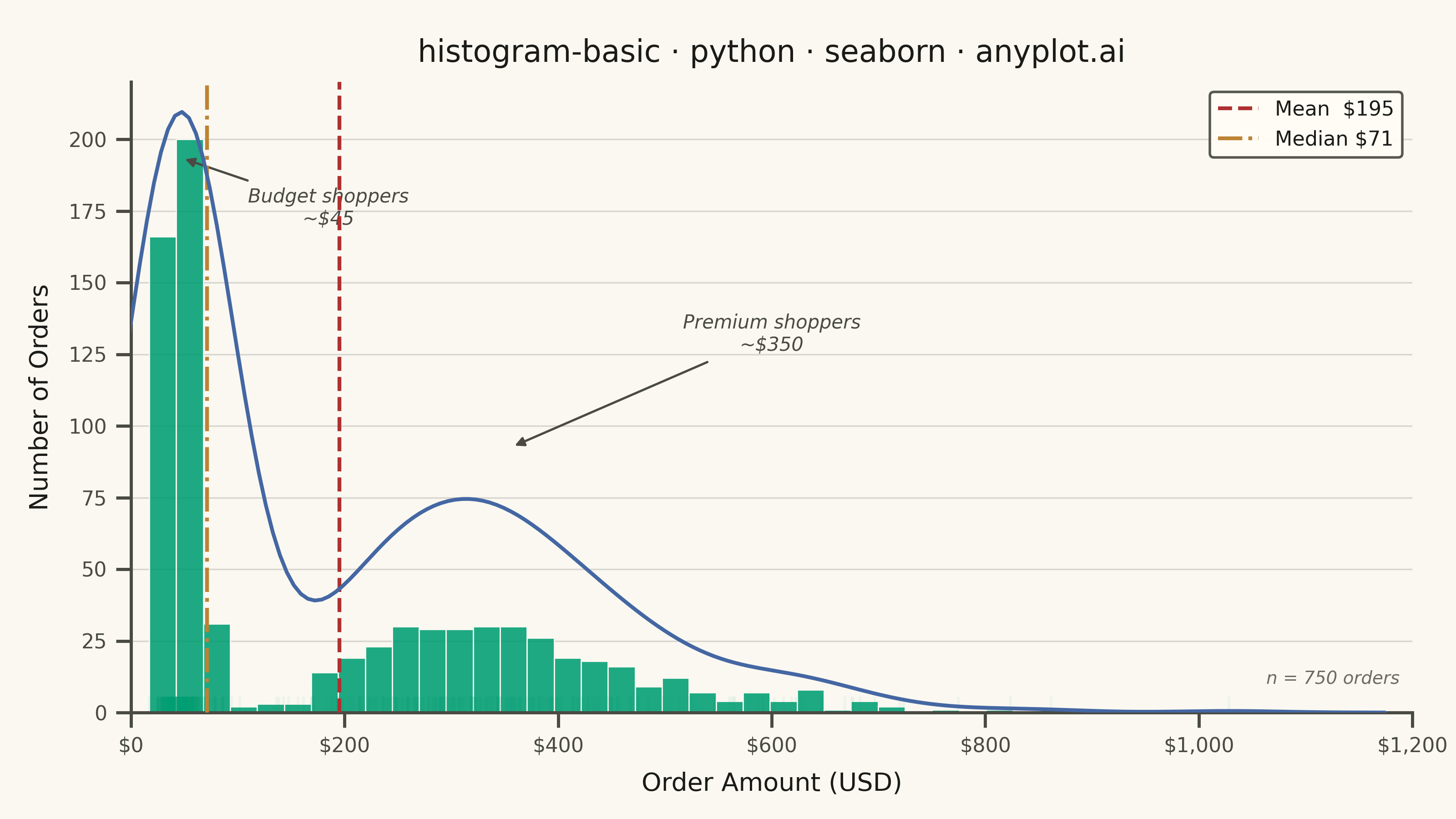
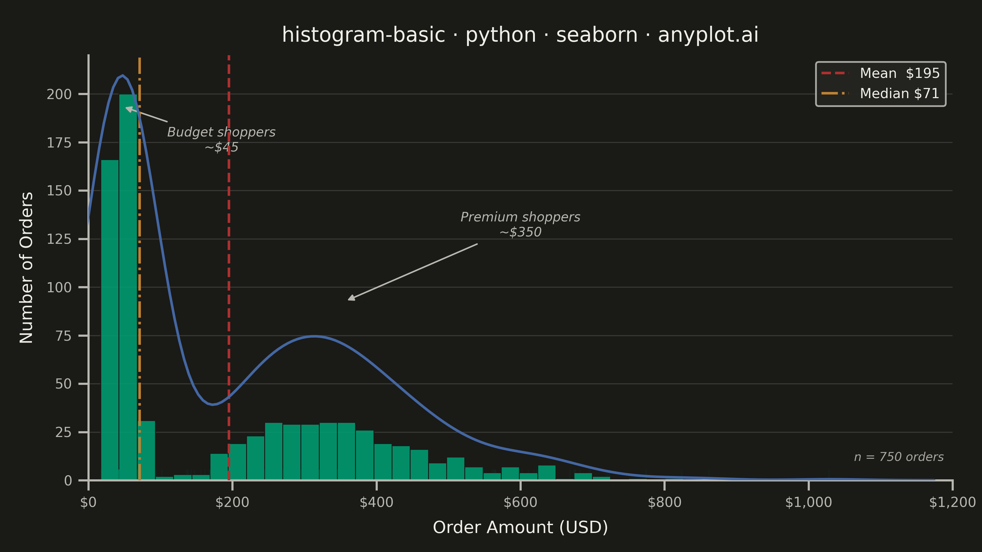
A histogram displays the distribution of a single continuous variable by dividing the data range into bins and showing the frequency (count) of observations in each bin. It reveals the shape of the data distribution, including central tendency, spread, and presence of outliers or multiple modes.
""" anyplot.ai
histogram-basic: Basic Histogram
Library: seaborn 0.13.2 | Python 3.13.13
Quality: 91/100 | Updated: 2026-05-28
"""

import os as _os
import sys


# Prevent the local matplotlib.py in this directory from shadowing the package
_script_dir = _os.path.realpath(_os.path.dirname(_os.path.abspath(__file__)))
sys.path[:] = [p for p in sys.path if _os.path.realpath(p if p else ".") != _script_dir]
del _script_dir, _os

import os

import matplotlib.pyplot as plt
import matplotlib.ticker as ticker
import numpy as np
import seaborn as sns


THEME = os.getenv("ANYPLOT_THEME", "light")

PAGE_BG = "#FAF8F1" if THEME == "light" else "#1A1A17"
ELEVATED_BG = "#FFFDF6" if THEME == "light" else "#242420"
INK = "#1A1A17" if THEME == "light" else "#F0EFE8"
INK_SOFT = "#4A4A44" if THEME == "light" else "#B8B7B0"
INK_MUTED = "#6B6A63" if THEME == "light" else "#A8A79F"

IMPRINT_PALETTE = ["#009E73", "#C475FD", "#4467A3", "#BD8233", "#AE3030", "#2ABCCD", "#954477", "#99B314"]
BRAND = IMPRINT_PALETTE[0]

# Data — e-commerce order amounts: two clearly separated spending segments
# Budget shoppers (~$45) and premium shoppers (~$350) produce a bimodal distribution;
# mean >> median due to the right tail, giving well-separated reference lines.
np.random.seed(42)
budget = np.random.lognormal(np.log(45), 0.3, 400)
premium = np.random.lognormal(np.log(350), 0.35, 350)
values = np.concatenate([budget, premium])
values = values[(values > 5) & (values <= 1200)]

mean_val = np.mean(values)
median_val = np.median(values)

sns.set_theme(
    style="ticks",
    rc={
        "figure.facecolor": PAGE_BG,
        "axes.facecolor": PAGE_BG,
        "axes.edgecolor": INK_SOFT,
        "axes.labelcolor": INK,
        "text.color": INK,
        "xtick.color": INK_SOFT,
        "ytick.color": INK_SOFT,
        "grid.color": INK,
        "grid.alpha": 0.15,
        "legend.facecolor": ELEVATED_BG,
        "legend.edgecolor": INK_SOFT,
    },
)

fig, ax = plt.subplots(figsize=(8, 4.5), dpi=400)

# Histogram
sns.histplot(values, bins=40, color=BRAND, edgecolor=PAGE_BG, linewidth=0.5, alpha=0.88, stat="count", ax=ax)

# KDE overlay via twin axis — seaborn-distinctive, shows both modes as humps
ax2 = ax.twinx()
sns.kdeplot(values, color=IMPRINT_PALETTE[2], linewidth=1.5, ax=ax2)
ax2.set_ylabel("")
ax2.set_yticks([])
for sp in ax2.spines.values():
    sp.set_visible(False)

# Rugplot — individual observations
sns.rugplot(values, color=BRAND, alpha=0.05, height=0.025, ax=ax)

# Reference lines for distributional statistics
mean_line = ax.axvline(mean_val, color=IMPRINT_PALETTE[4], linewidth=1.5, linestyle="--", zorder=5)
med_line = ax.axvline(median_val, color=IMPRINT_PALETTE[3], linewidth=1.5, linestyle="-.", zorder=5)

y_top = ax.get_ylim()[1]

# Mode annotations: text placed in the gap between peaks, arrows point to peak tops
ax.annotate(
    "Budget shoppers\n~$45",
    xy=(46, y_top * 0.88),
    xytext=(185, y_top * 0.80),
    fontsize=7.5,
    fontstyle="italic",
    color=INK_SOFT,
    ha="center",
    va="center",
    arrowprops={"arrowstyle": "-|>", "color": INK_SOFT, "lw": 0.9},
)
ax.annotate(
    "Premium shoppers\n~$350",
    xy=(355, y_top * 0.42),
    xytext=(600, y_top * 0.60),
    fontsize=7.5,
    fontstyle="italic",
    color=INK_SOFT,
    ha="center",
    va="center",
    arrowprops={"arrowstyle": "-|>", "color": INK_SOFT, "lw": 0.9},
)

# Legend labels reference lines in the sparse upper-right region
ax.legend(
    [mean_line, med_line],
    [f"Mean  ${mean_val:.0f}", f"Median ${median_val:.0f}"],
    fontsize=8,
    loc="upper right",
    facecolor=ELEVATED_BG,
    edgecolor=INK_SOFT,
    framealpha=0.92,
)

# Typography
ax.set_title("histogram-basic · python · seaborn · anyplot.ai", fontsize=12, fontweight="medium", color=INK, pad=8)
ax.set_xlabel("Order Amount (USD)", fontsize=10, color=INK, labelpad=6)
ax.set_ylabel("Number of Orders", fontsize=10, color=INK, labelpad=6)
ax.tick_params(axis="both", labelsize=8, colors=INK_SOFT)

# X-axis dollar formatting
ax.xaxis.set_major_formatter(ticker.FuncFormatter(lambda x, _: f"${int(x):,}"))
ax.xaxis.set_major_locator(ticker.MultipleLocator(200))

ax.set_xlim(0, 1200)
ax.set_ylim(bottom=0)
ax.spines["top"].set_visible(False)
ax.spines["right"].set_visible(False)
ax.yaxis.grid(True, alpha=0.15, linewidth=0.6, color=INK)
ax.xaxis.grid(False)

# Sample size footnote (lower-right, clear of annotations)
ax.text(
    0.99,
    0.04,
    f"n = {len(values):,} orders",
    transform=ax.transAxes,
    fontsize=7,
    color=INK_MUTED,
    ha="right",
    va="bottom",
    fontstyle="italic",
)

fig.subplots_adjust(left=0.09, right=0.97, top=0.90, bottom=0.13)
plt.savefig(f"plot-{THEME}.png", dpi=400, facecolor=PAGE_BG)
plt.close()
Runnable source as JSON, for any HTTP client: https://api.anyplot.ai/specs/histogram-basic/seaborn/code. Any spec id and library id listed in llms-full.txt fit the same URL shape; every URL below is complete and callable.
{
  "spec_id": "histogram-basic",
  "language": "python",
  "library": "seaborn",
  "page": "https://anyplot.ai/histogram-basic/python/seaborn",
  "hub": "https://anyplot.ai/histogram-basic",
  "code_json": "https://api.anyplot.ai/specs/histogram-basic/seaborn/code",
  "spec_json": "https://api.anyplot.ai/specs/histogram-basic",
  "render_light_png": "https://storage.googleapis.com/anyplot-images/plots/histogram-basic/python/seaborn/plot-light.png",
  "render_dark_png": "https://storage.googleapis.com/anyplot-images/plots/histogram-basic/python/seaborn/plot-dark.png",
  "quality_score": 91.0,
  "license": "MIT",
  "guide": "https://anyplot.ai/llms.txt"
}
Part of Basic Histogram on anyplot.ai.