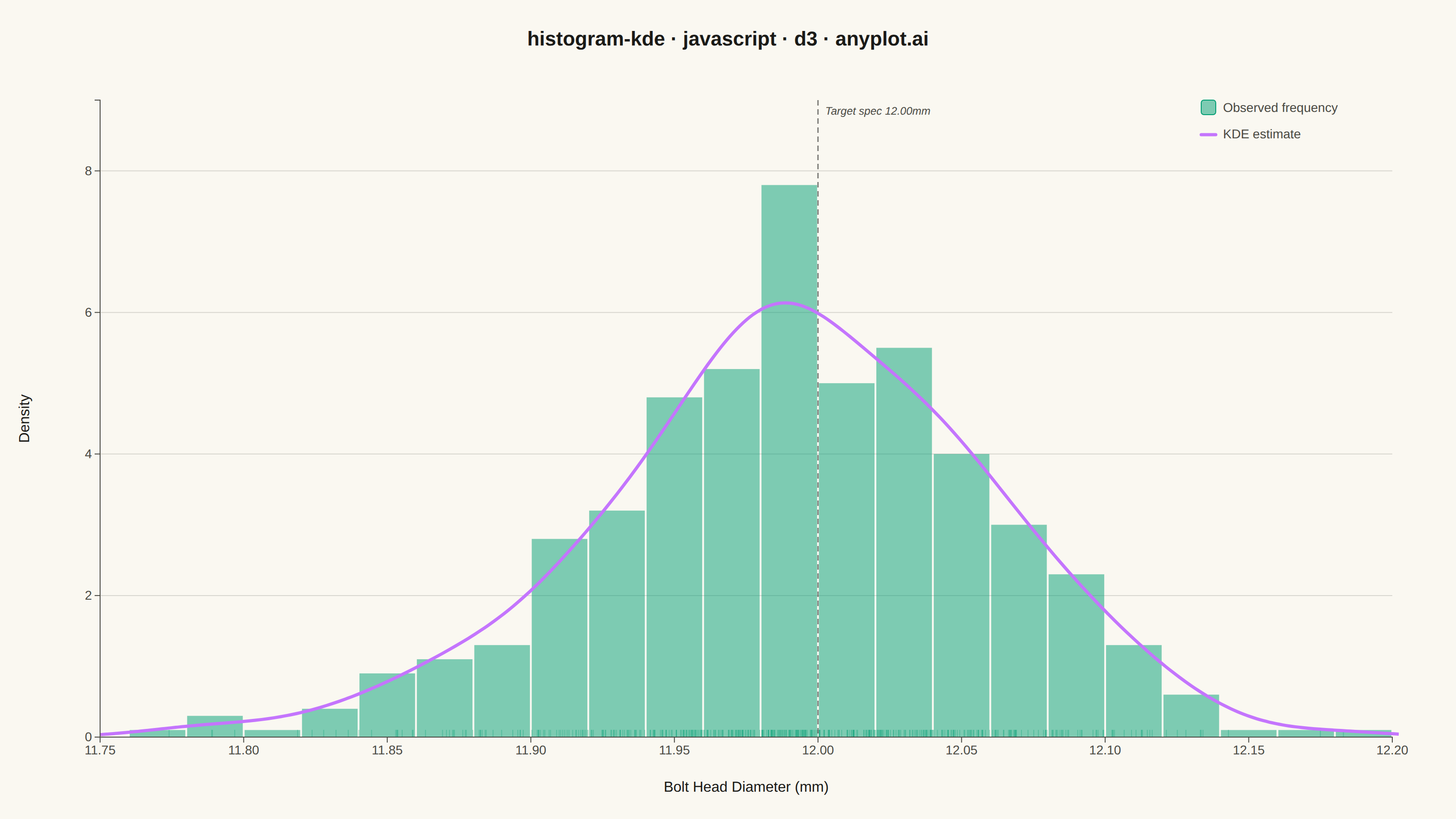
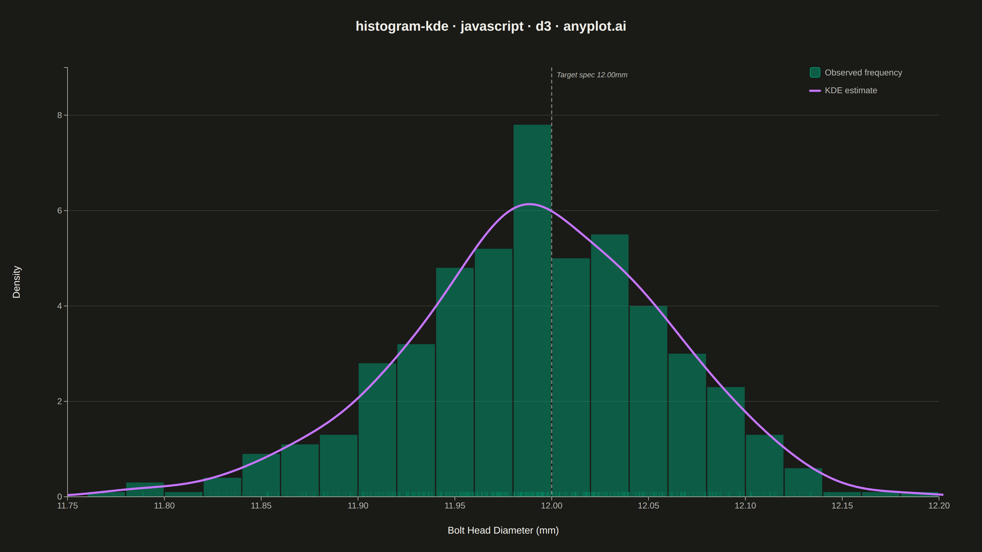
A histogram with kernel density estimate (KDE) overlay combines discrete binning with continuous density estimation to visualize the distribution of continuous data. The histogram bars show frequency counts in each bin while the smooth KDE curve reveals the underlying probability density, making it easier to perceive the true shape of the distribution without binning artifacts.
// anyplot.ai
// histogram-kde: Histogram with KDE Overlay
// Library: d3 7.9.0 | JavaScript 22.23.1
// Quality: 89/100 | Created: 2026-08-05

const t = window.ANYPLOT_TOKENS;
const { width, height } = window.ANYPLOT_SIZE;
const margin = { top: 110, right: 70, bottom: 90, left: 110 };
const iw = width - margin.left - margin.right;
const ih = height - margin.top - margin.bottom;

// --- Data (in-memory, deterministic) ----------------------------------------
// Bolt head diameter measurements from a QC gauge station (target spec 12.00mm).
// A tiny fixed-seed LCG stands in for the browser's lack of a seeded RNG.
function lcg(seed) {
  let state = seed;
  return () => {
    state = (state * 1664525 + 1013904223) % 4294967296;
    return state / 4294967296;
  };
}
const rand = lcg(42);
function randNormal() {
  const u1 = Math.max(rand(), 1e-9);
  const u2 = rand();
  return Math.sqrt(-2 * Math.log(u1)) * Math.cos(2 * Math.PI * u2);
}

const n = 500;
const diameters = [];
for (let i = 0; i < n; i++) {
  // 90% of parts cluster tightly on the target; 10% come from a slightly
  // undersized secondary mode (early tool wear), pulling the tail left.
  const drifted = rand() < 0.1;
  const mean = drifted ? 11.86 : 12.0;
  const std = drifted ? 0.05 : 0.06;
  diameters.push(mean + std * randNormal());
}

const mean = d3.mean(diameters);
const std = d3.deviation(diameters);

// --- Scales -------------------------------------------------------------
const x = d3.scaleLinear().domain(d3.extent(diameters)).nice().range([0, iw]);

const bins = d3.bin().domain(x.domain()).thresholds(30)(diameters);
const histDensity = bins.map((b) => ({
  x0: b.x0,
  x1: b.x1,
  density: b.length / (n * (b.x1 - b.x0)),
}));

const bandwidth = 1.06 * std * Math.pow(n, -0.2);
function gaussianKernel(bw) {
  return (u) => Math.exp(-0.5 * (u / bw) ** 2) / (bw * Math.sqrt(2 * Math.PI));
}
const kernel = gaussianKernel(bandwidth);
const [xMin, xMax] = x.domain();
const grid = d3.range(xMin, xMax + (xMax - xMin) / 200, (xMax - xMin) / 200);
const kde = grid.map((gx) => [gx, d3.mean(diameters, (v) => kernel(gx - v))]);

const yMax = Math.max(d3.max(histDensity, (d) => d.density), d3.max(kde, (d) => d[1]));
const y = d3.scaleLinear().domain([0, yMax * 1.08]).nice().range([ih, 0]);

// --- SVG mount ------------------------------------------------------------
const svg = d3.select("#container").append("svg").attr("width", width).attr("height", height);
const g = svg.append("g").attr("transform", `translate(${margin.left},${margin.top})`);

// --- Gridlines (y-axis only) -----------------------------------------------
g.append("g")
  .attr("class", "grid")
  .call(d3.axisLeft(y).ticks(6).tickSize(-iw).tickFormat(""))
  .call((sel) => sel.select(".domain").remove())
  .selectAll("line")
  .attr("stroke", t.grid);

// --- Histogram bars (density-scaled) ----------------------------------------
g.selectAll(".bar")
  .data(histDensity)
  .join("rect")
  .attr("class", "bar")
  .attr("x", (d) => x(d.x0) + 1)
  .attr("y", (d) => y(d.density))
  .attr("width", (d) => Math.max(0, x(d.x1) - x(d.x0) - 2))
  .attr("height", (d) => ih - y(d.density))
  .attr("fill", t.palette[0])
  .attr("fill-opacity", 0.5);

// --- Rug (raw observations along the x-axis baseline) -----------------------
g.selectAll(".rug")
  .data(diameters)
  .join("line")
  .attr("class", "rug")
  .attr("x1", (d) => x(d))
  .attr("x2", (d) => x(d))
  .attr("y1", ih)
  .attr("y2", ih - 8)
  .attr("stroke", t.palette[0])
  .attr("stroke-width", 1)
  .attr("stroke-opacity", 0.3);

// --- Target spec reference line (12.00mm) ------------------------------
const targetX = x(12.0);
g.append("line")
  .attr("x1", targetX)
  .attr("x2", targetX)
  .attr("y1", 0)
  .attr("y2", ih)
  .attr("stroke", t.ink)
  .attr("stroke-width", 1.5)
  .attr("stroke-dasharray", "6,4")
  .attr("stroke-opacity", 0.55);
g.append("text")
  .attr("x", targetX + 8)
  .attr("y", 16)
  .attr("fill", t.inkSoft)
  .style("font-size", "12px")
  .style("font-style", "italic")
  .text("Target spec 12.00mm");

// --- KDE curve ---------------------------------------------------------
const line = d3
  .line()
  .x((d) => x(d[0]))
  .y((d) => y(d[1]))
  .curve(d3.curveNatural);

g.append("path").datum(kde).attr("fill", "none").attr("stroke", t.palette[1]).attr("stroke-width", 3.5).attr("d", line);

// --- Axes -------------------------------------------------------------------
const xAxis = g
  .append("g")
  .attr("transform", `translate(0,${ih})`)
  .call(d3.axisBottom(x).ticks(8).tickFormat((d) => d.toFixed(2)));
const yAxis = g.append("g").call(d3.axisLeft(y).ticks(6));
for (const ax of [xAxis, yAxis]) {
  ax.selectAll("text").attr("fill", t.inkSoft).style("font-size", "14px");
  ax.selectAll("line").attr("stroke", t.inkSoft);
  ax.select(".domain").attr("stroke", t.inkSoft);
}

// --- Axis labels --------------------------------------------------------
g.append("text")
  .attr("x", iw / 2)
  .attr("y", ih + 60)
  .attr("text-anchor", "middle")
  .attr("fill", t.ink)
  .style("font-size", "16px")
  .text("Bolt Head Diameter (mm)");

g.append("text")
  .attr("transform", "rotate(-90)")
  .attr("x", -ih / 2)
  .attr("y", -78)
  .attr("text-anchor", "middle")
  .attr("fill", t.ink)
  .style("font-size", "16px")
  .text("Density");

// --- Legend -------------------------------------------------------------
const legend = g.append("g").attr("transform", `translate(${iw - 210},0)`);
legend
  .append("rect")
  .attr("x", 0)
  .attr("y", 0)
  .attr("width", 16)
  .attr("height", 16)
  .attr("rx", 3)
  .attr("ry", 3)
  .attr("fill", t.palette[0])
  .attr("fill-opacity", 0.5)
  .attr("stroke", t.palette[0])
  .attr("stroke-width", 1);
legend.append("text").attr("x", 24).attr("y", 13).attr("fill", t.inkSoft).style("font-size", "14px").text("Observed frequency");
legend
  .append("line")
  .attr("x1", 0)
  .attr("y1", 38)
  .attr("x2", 16)
  .attr("y2", 38)
  .attr("stroke", t.palette[1])
  .attr("stroke-width", 3.5)
  .attr("stroke-linecap", "round");
legend.append("text").attr("x", 24).attr("y", 42).attr("fill", t.inkSoft).style("font-size", "14px").text("KDE estimate");

// --- Title --------------------------------------------------------------
svg
  .append("text")
  .attr("x", width / 2)
  .attr("y", 50)
  .attr("text-anchor", "middle")
  .attr("fill", t.ink)
  .style("font-size", "22px")
  .style("font-weight", "600")
  .text("histogram-kde · javascript · d3 · anyplot.ai");
Runnable source as JSON, for any HTTP client: https://api.anyplot.ai/specs/histogram-kde/d3/code. Any spec id and library id listed in llms-full.txt fit the same URL shape; every URL below is complete and callable.
{
  "spec_id": "histogram-kde",
  "language": "javascript",
  "library": "d3",
  "page": "https://anyplot.ai/histogram-kde/javascript/d3",
  "hub": "https://anyplot.ai/histogram-kde",
  "code_json": "https://api.anyplot.ai/specs/histogram-kde/d3/code",
  "spec_json": "https://api.anyplot.ai/specs/histogram-kde",
  "render_light_png": "https://storage.googleapis.com/anyplot-images/plots/histogram-kde/javascript/d3/plot-light.png",
  "render_dark_png": "https://storage.googleapis.com/anyplot-images/plots/histogram-kde/javascript/d3/plot-dark.png",
  "interactive_light_html": "https://storage.googleapis.com/anyplot-images/plots/histogram-kde/javascript/d3/plot-light.html",
  "interactive_dark_html": "https://storage.googleapis.com/anyplot-images/plots/histogram-kde/javascript/d3/plot-dark.html",
  "quality_score": 89.0,
  "license": "MIT",
  "guide": "https://anyplot.ai/llms.txt"
}
Part of Histogram with KDE Overlay on anyplot.ai.