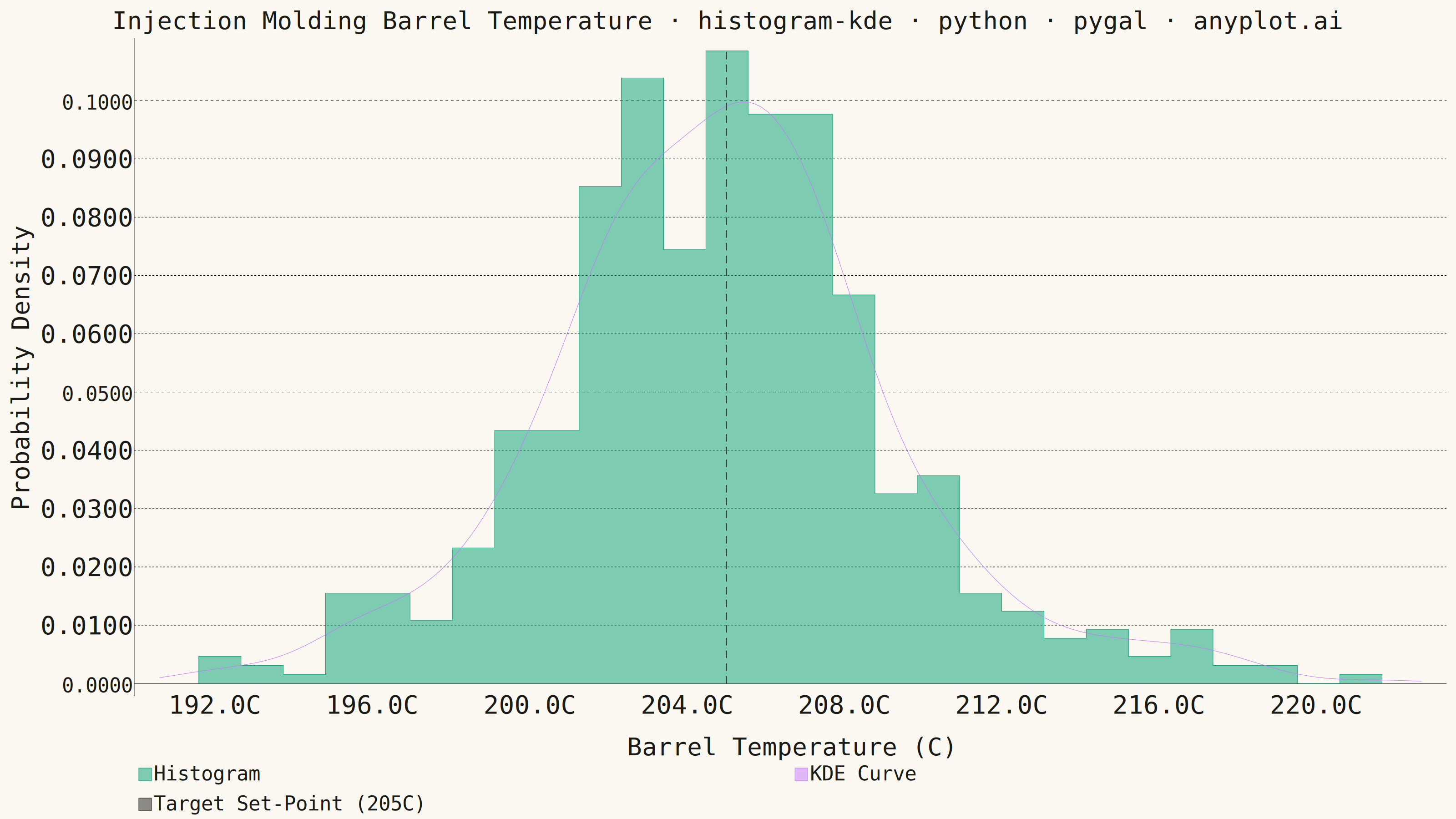
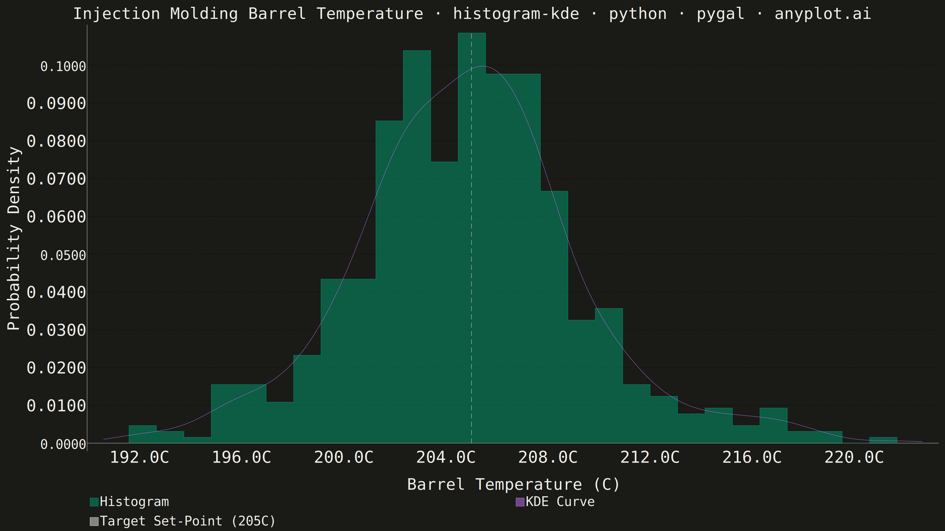
A histogram with kernel density estimate (KDE) overlay combines discrete binning with continuous density estimation to visualize the distribution of continuous data. The histogram bars show frequency counts in each bin while the smooth KDE curve reveals the underlying probability density, making it easier to perceive the true shape of the distribution without binning artifacts.
""" anyplot.ai
histogram-kde: Histogram with KDE Overlay
Library: pygal 3.1.3 | Python 3.13.14
Quality: 87/100 | Updated: 2026-08-05
"""

import os

import numpy as np
import pygal
from pygal.style import Style


# Theme tokens (see prompts/default-style-guide.md "Theme-adaptive Chrome")
THEME = os.getenv("ANYPLOT_THEME", "light")
PAGE_BG = "#FAF8F1" if THEME == "light" else "#1A1A17"
INK = "#1A1A17" if THEME == "light" else "#F0EFE8"
INK_MUTED = "#6B6A63" if THEME == "light" else "#A8A79F"

# Imprint categorical palette (canonical order, first series always #009E73)
IMPRINT_PALETTE = (
    "#009E73",  # brand green — histogram bars
    "#C475FD",  # lavender — KDE curve
    "#4467A3",  # blue
    "#BD8233",  # ochre
    "#AE3030",  # matte red
    "#2ABCCD",  # cyan
    "#954477",  # rose
    "#99B314",  # lime
)

# Data - injection molding barrel temperature readings from a quality-control
# monitoring line, target set-point 205C, with occasional cold-start and
# overheat excursions that give the distribution its tail behavior
np.random.seed(42)
temperatures = np.concatenate(
    [
        np.random.normal(205, 3.5, 550),  # steady-state process operation
        np.random.normal(196, 2.0, 30),  # cold-start under-temp events
        np.random.normal(216, 2.5, 20),  # overheat spikes
    ]
)

# Compute histogram bins with density normalization
n_bins = 28
counts, bin_edges = np.histogram(temperatures, bins=n_bins, density=True)

# Compute KDE using a Gaussian kernel (Scott's rule for bandwidth)
x_range = np.linspace(temperatures.min() - 1, temperatures.max() + 1, 200)
n = len(temperatures)
bandwidth = n ** (-1 / 5) * np.std(temperatures)
kde = np.zeros_like(x_range)
for xi in temperatures:
    kde += np.exp(-0.5 * ((x_range - xi) / bandwidth) ** 2)
kde /= n * bandwidth * np.sqrt(2 * np.pi)

# Histogram bars as a filled step path so pygal's XY chart can draw them
hist_xy = [(float(bin_edges[0]), 0.0)]
for i, count in enumerate(counts):
    left = float(bin_edges[i])
    right = float(bin_edges[i + 1])
    height = float(count)
    hist_xy.append((left, height))
    hist_xy.append((right, height))
hist_xy.append((float(bin_edges[-1]), 0.0))

# Reference line at the 205C target set-point, spanning from the baseline up
# to the tallest peak so it reads as a data-storytelling cue without
# stretching the y-axis beyond what the histogram/KDE already require
target_temp = 205.0
target_height = float(max(counts.max(), kde.max()))
target_xy = [(target_temp, 0.0), (target_temp, target_height)]

# Title fontsize scales with the mandated title length (see
# prompts/plot-generator.md "Title fontsize must scale with title length")
title = "Injection Molding Barrel Temperature · histogram-kde · python · pygal · anyplot.ai"
title_font_size = max(round(66 * min(1.0, 67 / len(title))), 44)

# Style for the 3200x1800 px canvas with theme-adaptive tokens
# (see prompts/library/pygal.md "Sizing + Theme for 3200x1800 px")
# Third series color is the "neutral" semantic anchor (same hex as INK) so the
# 205C reference line reads as chart structure rather than a fourth data category
custom_style = Style(
    background=PAGE_BG,
    plot_background=PAGE_BG,
    foreground=INK,
    foreground_strong=INK,
    foreground_subtle=INK_MUTED,
    colors=(IMPRINT_PALETTE[0], IMPRINT_PALETTE[1], INK),
    title_font_size=title_font_size,
    label_font_size=56,
    major_label_font_size=44,
    legend_font_size=44,
    value_font_size=36,
    opacity=0.5,
    opacity_hover=0.7,
    stroke_opacity=1,
)

# Create XY chart. Pygal-distinctive tooltip formatters give the interactive
# HTML export readable hover values (temperature in C, density to 4 decimals)
# without touching the static PNG.
chart = pygal.XY(
    width=3200,
    height=1800,
    style=custom_style,
    title=title,
    x_title="Barrel Temperature (C)",
    y_title="Probability Density",
    show_dots=False,
    show_legend=True,
    legend_at_bottom=True,
    legend_box_size=28,
    show_y_guides=True,
    show_x_guides=False,
    x_value_formatter=lambda x: f"{x:.1f}C",
    value_formatter=lambda y: f"{y:.4f}",
)

# Semi-transparent histogram fill (first series, brand green) so the KDE
# curve remains visible through the bars
chart.add("Histogram", hist_xy, fill=True, stroke_style={"width": 2.5})

# KDE curve drawn thick and fully opaque so it stays prominent over the
# tallest green peaks in both themes (second series, lavender)
kde_data = [(float(x), float(y)) for x, y in zip(x_range, kde, strict=True)]
chart.add("KDE Curve", kde_data, fill=False, stroke_style={"width": 8})

# Dashed neutral-tone reference line calling out the 205C target set-point,
# turning the plot from a plain distribution into a QC story about how far
# the cold-start/overheat tails drift from spec (third series)
chart.add(
    "Target Set-Point (205C)",
    target_xy,
    fill=False,
    stroke_style={"width": 3, "dasharray": "16, 12", "linecap": "round"},
)

# Save outputs
chart.render_to_file(f"plot-{THEME}.html")
chart.render_to_png(f"plot-{THEME}.png")
Runnable source as JSON, for any HTTP client: https://api.anyplot.ai/specs/histogram-kde/pygal/code. Any spec id and library id listed in llms-full.txt fit the same URL shape; every URL below is complete and callable.
{
  "spec_id": "histogram-kde",
  "language": "python",
  "library": "pygal",
  "page": "https://anyplot.ai/histogram-kde/python/pygal",
  "hub": "https://anyplot.ai/histogram-kde",
  "code_json": "https://api.anyplot.ai/specs/histogram-kde/pygal/code",
  "spec_json": "https://api.anyplot.ai/specs/histogram-kde",
  "render_light_png": "https://storage.googleapis.com/anyplot-images/plots/histogram-kde/python/pygal/plot-light.png",
  "render_dark_png": "https://storage.googleapis.com/anyplot-images/plots/histogram-kde/python/pygal/plot-dark.png",
  "interactive_light_html": "https://storage.googleapis.com/anyplot-images/plots/histogram-kde/python/pygal/plot-light.html",
  "interactive_dark_html": "https://storage.googleapis.com/anyplot-images/plots/histogram-kde/python/pygal/plot-dark.html",
  "quality_score": 87.0,
  "license": "MIT",
  "guide": "https://anyplot.ai/llms.txt"
}
Part of Histogram with KDE Overlay on anyplot.ai.