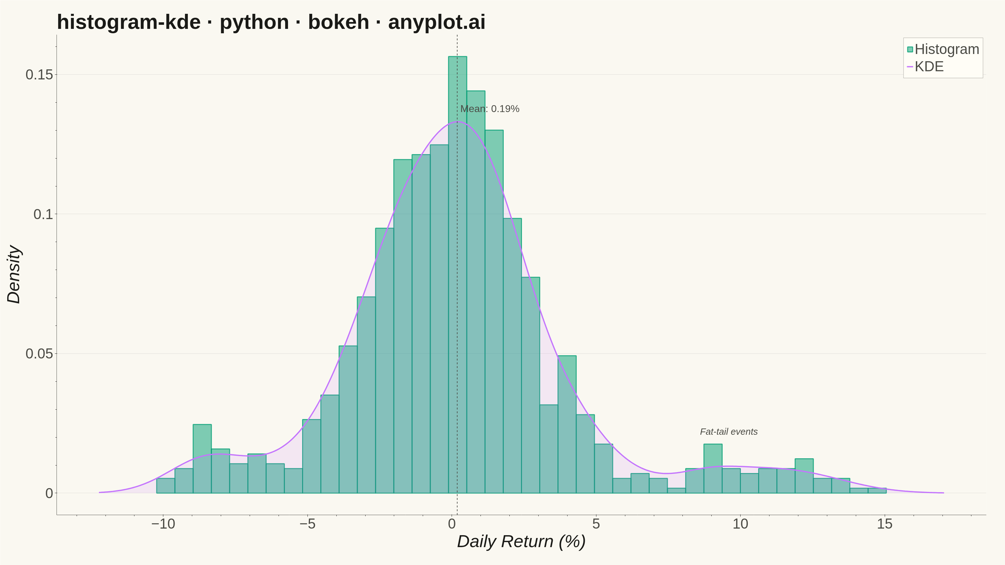
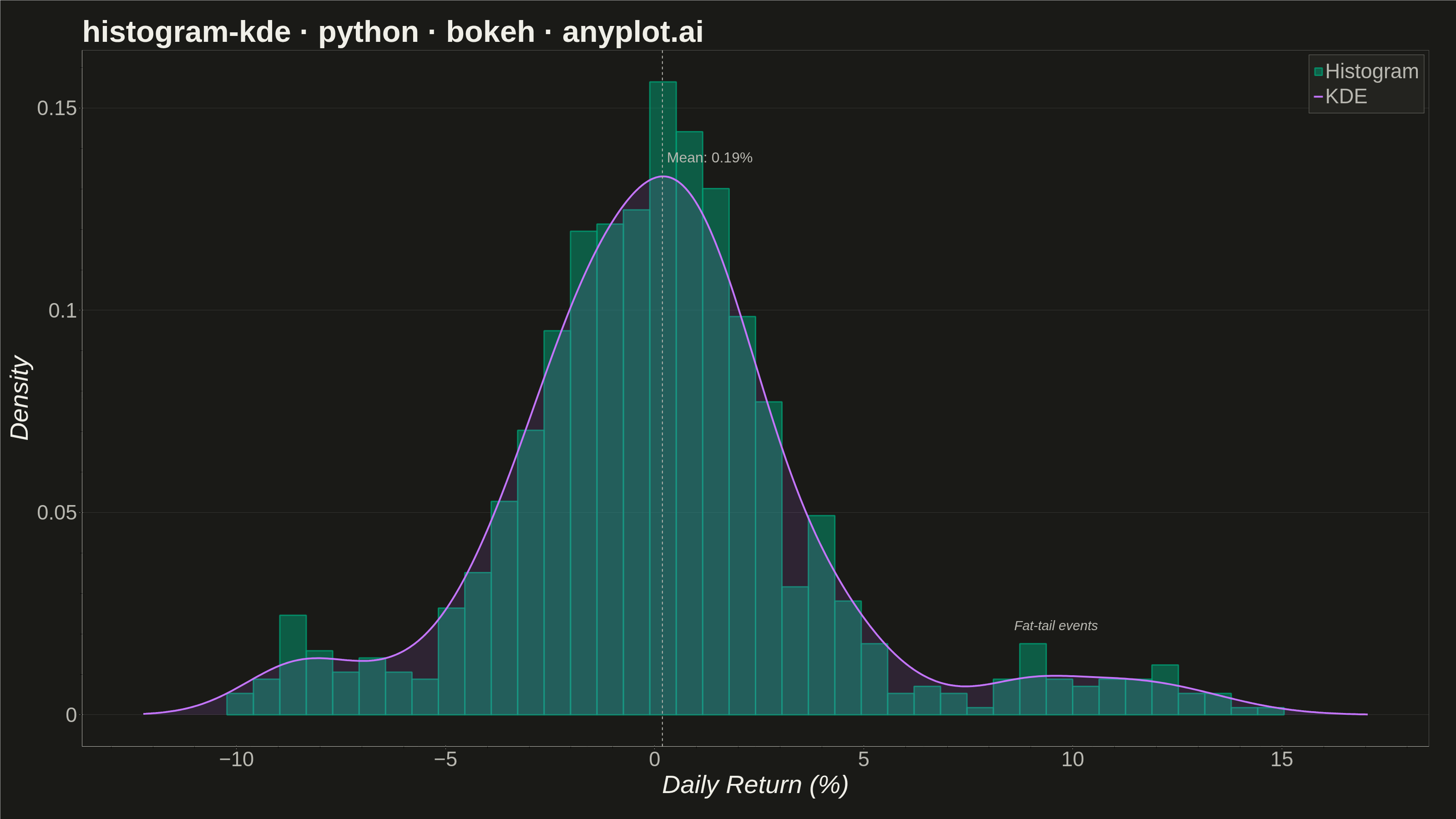
A histogram with kernel density estimate (KDE) overlay combines discrete binning with continuous density estimation to visualize the distribution of continuous data. The histogram bars show frequency counts in each bin while the smooth KDE curve reveals the underlying probability density, making it easier to perceive the true shape of the distribution without binning artifacts.
""" anyplot.ai
histogram-kde: Histogram with KDE Overlay
Library: bokeh 3.9.2 | Python 3.13.14
Quality: 91/100 | Updated: 2026-08-05
"""

import os
import sys
import time
from pathlib import Path

import numpy as np


# Remove current directory from path to avoid importing bokeh.py instead of bokeh package
script_dir = os.path.dirname(os.path.abspath(__file__)) if "__file__" in globals() else os.getcwd()
if sys.path and sys.path[0] in ("", ".", script_dir):
    sys.path.pop(0)

# Change to script directory to save output files there
os.chdir(script_dir)

from bokeh.io import output_file, save
from bokeh.models import ColumnDataSource, HoverTool, Label, Span
from bokeh.plotting import figure
from selenium import webdriver
from selenium.webdriver.chrome.options import Options


# Theme setup
THEME = os.getenv("ANYPLOT_THEME", "light")
PAGE_BG = "#FAF8F1" if THEME == "light" else "#1A1A17"
ELEVATED_BG = "#FFFDF6" if THEME == "light" else "#242420"
INK = "#1A1A17" if THEME == "light" else "#F0EFE8"
INK_SOFT = "#4A4A44" if THEME == "light" else "#B8B7B0"

# Imprint palette (first series always #009E73)
HISTOGRAM_COLOR = "#009E73"  # Imprint palette position 1
KDE_COLOR = "#C475FD"  # Imprint palette position 2

# Data - Simulating stock returns distribution (realistic financial data)
np.random.seed(42)
# Mix of normal market conditions and some fat-tail events
main_returns = np.random.normal(0.05, 2.5, 800)  # Daily returns in %
tail_events = np.concatenate(
    [
        np.random.normal(-8, 1.5, 50),  # Negative tail events
        np.random.normal(10, 2, 50),  # Positive tail events
    ]
)
values = np.concatenate([main_returns, tail_events])

# Histogram computation (density-normalized)
bin_count = 40
hist, bin_edges = np.histogram(values, bins=bin_count, density=True)

# KDE computation using Gaussian kernel (Scott's rule bandwidth)
x_kde = np.linspace(values.min() - 2, values.max() + 2, 500)
bandwidth = 1.06 * np.std(values) * len(values) ** (-1 / 5)
y_kde = np.zeros_like(x_kde)
for xi in values:
    y_kde += np.exp(-0.5 * ((x_kde - xi) / bandwidth) ** 2)
y_kde /= len(values) * bandwidth * np.sqrt(2 * np.pi)
mean_return = float(np.mean(values))

# Create figure — toolbar_location=None prevents extra height above the canvas
hist_hover = HoverTool(tooltips=[("Range", "@left{0.00} - @right{0.00}"), ("Density", "@top{0.00}")])
p = figure(
    width=3200,
    height=1800,
    title="histogram-kde · python · bokeh · anyplot.ai",
    x_axis_label="Daily Return (%)",
    y_axis_label="Density",
    toolbar_location=None,
    tools=[hist_hover],
    min_border_bottom=160,
    min_border_left=180,
    min_border_top=110,
    min_border_right=60,
)

# Histogram using quad glyphs
hist_source = ColumnDataSource(
    data={"left": bin_edges[:-1], "right": bin_edges[1:], "top": hist, "bottom": [0] * len(hist)}
)

p.quad(
    left="left",
    right="right",
    top="top",
    bottom="bottom",
    source=hist_source,
    fill_color=HISTOGRAM_COLOR,
    fill_alpha=0.5,
    line_color=HISTOGRAM_COLOR,
    line_alpha=0.8,
    line_width=3,
    legend_label="Histogram",
)

# KDE curve — subtle area fill beneath the line adds depth without hiding the histogram
kde_source = ColumnDataSource(data={"x": x_kde, "y": y_kde})
p.varea(x="x", y1=0, y2="y", source=kde_source, fill_color=KDE_COLOR, fill_alpha=0.12)
p.line(x="x", y="y", source=kde_source, line_color=KDE_COLOR, line_width=4, legend_label="KDE")

# Mean marker — dashed reference line gives the reader an immediate focal point
mean_span = Span(location=mean_return, dimension="height", line_color=INK_SOFT, line_dash="dashed", line_width=2)
p.add_layout(mean_span)
mean_label = Label(
    x=mean_return,
    y=float(y_kde.max()) * 1.02,
    text=f"Mean: {mean_return:.2f}%",
    text_font_size="24pt",
    text_color=INK_SOFT,
    x_offset=10,
)
p.add_layout(mean_label)

# Fat-tail annotation — calls out the positive tail bump to sharpen the
# visual story beyond the single mean-line focal point
tail_mask = x_kde > 8
tail_peak_idx = np.where(tail_mask)[0][np.argmax(y_kde[tail_mask])]
tail_peak_x = float(x_kde[tail_peak_idx])
tail_peak_y = float(y_kde[tail_peak_idx])
tail_label = Label(
    x=tail_peak_x,
    y=tail_peak_y + float(y_kde.max()) * 0.08,
    text="Fat-tail events",
    text_font_size="22pt",
    text_font_style="italic",
    text_color=INK_SOFT,
    text_align="center",
)
p.add_layout(tail_label)

# Add hover tool for KDE curve
kde_hover = HoverTool(tooltips=[("Return (%)", "@x{0.00}"), ("Density", "@y{0.0000}")])
p.add_tools(kde_hover)

# Title styling
p.title.text_font_size = "50pt"
p.title.text_color = INK

# Axis styling (canonical 3200x1800 sizing)
p.xaxis.axis_label_text_font_size = "42pt"
p.yaxis.axis_label_text_font_size = "42pt"
p.xaxis.axis_label_text_color = INK
p.yaxis.axis_label_text_color = INK
p.xaxis.major_label_text_font_size = "34pt"
p.yaxis.major_label_text_font_size = "34pt"
p.xaxis.major_label_text_color = INK_SOFT
p.yaxis.major_label_text_color = INK_SOFT

# Grid styling - horizontal only, subtle (vertical grid adds no value across histogram bins)
p.xgrid.grid_line_color = None
p.ygrid.grid_line_color = INK
p.ygrid.grid_line_alpha = 0.12

# Legend styling
p.legend.label_text_font_size = "34pt"
p.legend.location = "top_right"
p.legend.background_fill_color = ELEVATED_BG
p.legend.border_line_color = INK_SOFT
p.legend.label_text_color = INK_SOFT

# Axis and border colors — no outline box, L-shaped frame via left/bottom axis lines only
p.background_fill_color = PAGE_BG
p.border_fill_color = PAGE_BG
p.outline_line_color = None
p.xaxis.axis_line_color = INK_SOFT
p.yaxis.axis_line_color = INK_SOFT
p.xaxis.major_tick_line_color = INK_SOFT
p.yaxis.major_tick_line_color = INK_SOFT

# Save as HTML
output_file(f"plot-{THEME}.html")
save(p)

# Screenshot with headless Chrome — Selenium 4 / Selenium Manager auto-resolves the driver
W, H = 3200, 1800
opts = Options()
for arg in (
    "--headless=new",
    "--no-sandbox",
    "--disable-dev-shm-usage",
    "--disable-gpu",
    f"--window-size={W},{H}",
    "--hide-scrollbars",
    "--force-device-scale-factor=1",
):
    opts.add_argument(arg)
driver = webdriver.Chrome(options=opts)
driver.set_window_size(W, H)
driver.get(f"file://{Path(f'plot-{THEME}.html').resolve()}")
# Headless Chrome's --window-size sets the OUTER window, which still reserves a
# phantom title-bar height even headless — pin the viewport exactly via CDP.
driver.execute_cdp_cmd(
    "Emulation.setDeviceMetricsOverride", {"width": W, "height": H, "deviceScaleFactor": 1, "mobile": False}
)
time.sleep(3)  # let bokeh's JS render the canvas
driver.save_screenshot(f"plot-{THEME}.png")
driver.quit()
Runnable source as JSON, for any HTTP client: https://api.anyplot.ai/specs/histogram-kde/bokeh/code. Any spec id and library id listed in llms-full.txt fit the same URL shape; every URL below is complete and callable.
{
  "spec_id": "histogram-kde",
  "language": "python",
  "library": "bokeh",
  "page": "https://anyplot.ai/histogram-kde/python/bokeh",
  "hub": "https://anyplot.ai/histogram-kde",
  "code_json": "https://api.anyplot.ai/specs/histogram-kde/bokeh/code",
  "spec_json": "https://api.anyplot.ai/specs/histogram-kde",
  "render_light_png": "https://storage.googleapis.com/anyplot-images/plots/histogram-kde/python/bokeh/plot-light.png",
  "render_dark_png": "https://storage.googleapis.com/anyplot-images/plots/histogram-kde/python/bokeh/plot-dark.png",
  "interactive_light_html": "https://storage.googleapis.com/anyplot-images/plots/histogram-kde/python/bokeh/plot-light.html",
  "interactive_dark_html": "https://storage.googleapis.com/anyplot-images/plots/histogram-kde/python/bokeh/plot-dark.html",
  "quality_score": 91.0,
  "license": "MIT",
  "guide": "https://anyplot.ai/llms.txt"
}
Part of Histogram with KDE Overlay on anyplot.ai.