The same plot in 14 other libraries — Python: Altair, Bokeh, lets-plot, Matplotlib, Plotly, plotnine, Pygal, Seaborn; Julia: Makie.jl; JavaScript: Chart.js, D3.js, Apache ECharts, Highcharts, MUI X Charts. Compare all 15 side by side: Innovation Radar with Time-Horizon Rings in Python, R, Julia and JavaScript.
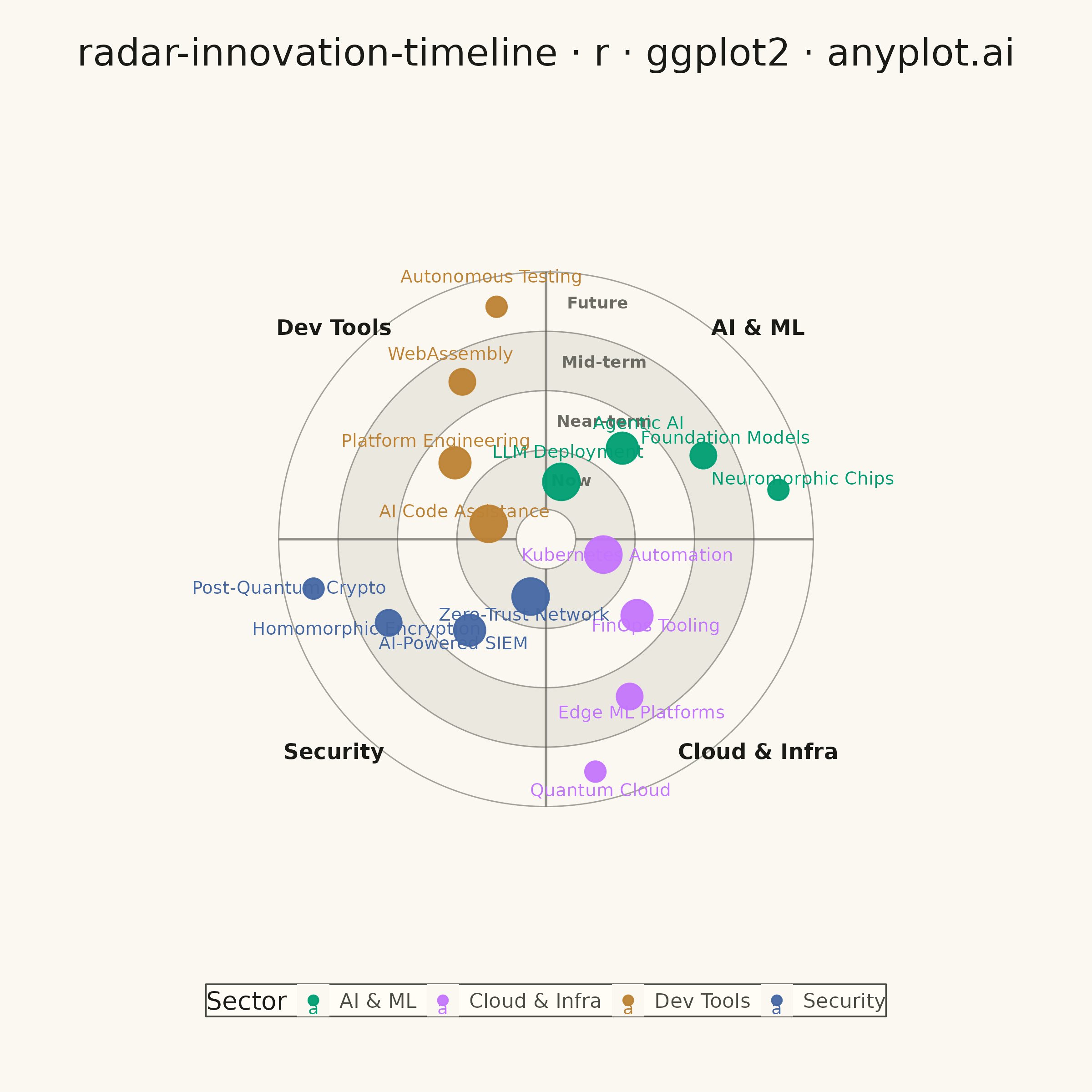
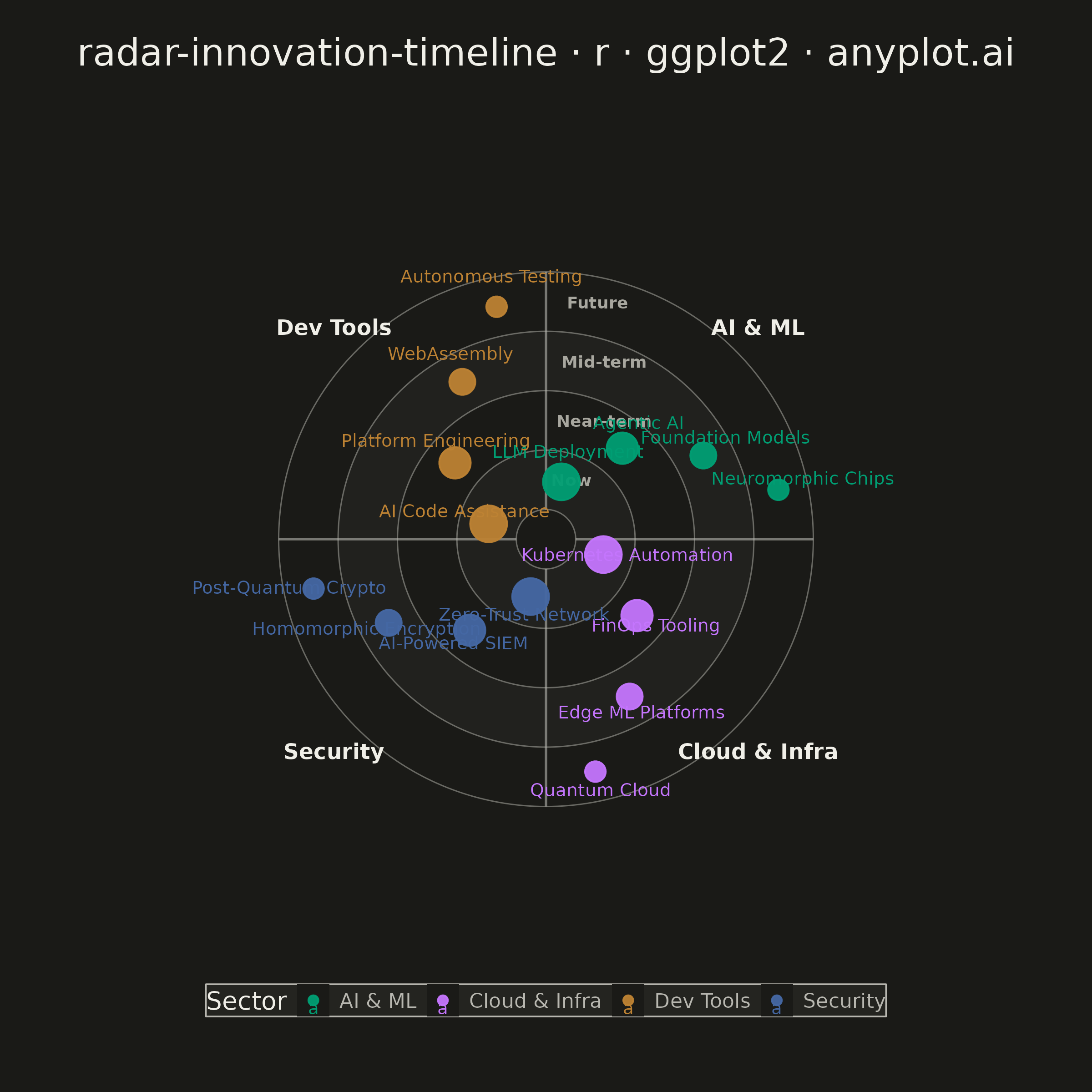
A radial chart that maps innovations, technologies, or trends onto concentric rings representing time horizons and angular sectors representing thematic categories. Inner rings represent near-term items (e.g., "Now", "Next 6 months") while outer rings represent longer-term or emerging trends (e.g., "2-5 years", "Future"). Each item is placed as a labeled point within its sector and ring, with distinct markers or colors encoding categories. Inspired by ThoughtWorks Technology Radar and similar strategic planning visualizations.
#' anyplot.ai
#' radar-innovation-timeline: Innovation Radar with Time-Horizon Rings
#' Library: ggplot2 3.5.1 | R 4.4.1
#' Quality: 80/100 | Created: 2026-05-29

library(ggplot2)
library(dplyr)
library(ragg)

set.seed(42)

# Theme tokens — Imprint palette
THEME       <- Sys.getenv("ANYPLOT_THEME", "light")
PAGE_BG     <- if (THEME == "light") "#FAF8F1" else "#1A1A17"
ELEVATED_BG <- if (THEME == "light") "#FFFDF6" else "#242420"
INK         <- if (THEME == "light") "#1A1A17" else "#F0EFE8"
INK_SOFT    <- if (THEME == "light") "#4A4A44" else "#B8B7B0"
INK_MUTED   <- if (THEME == "light") "#6B6A63" else "#A8A79F"

IMPRINT_PALETTE <- c(
  "#009E73",  # 1 — brand green → AI & ML
  "#C475FD",  # 2 — lavender    → Cloud & Infra
  "#4467A3",  # 3 — blue        → Security
  "#BD8233"   # 4 — ochre       → Dev Tools
)

sector_names  <- c("AI & ML", "Cloud & Infra", "Security", "Dev Tools")
ring_labels_v <- c("Now", "Near-term", "Mid-term", "Future")
color_map     <- setNames(IMPRINT_PALETTE, sector_names)
sector_starts <- setNames(c(0, 90, 180, 270), sector_names)

# 16 technology items: one per (sector × ring) cell
items <- tibble::tibble(
  name = c(
    "LLM Deployment", "Agentic AI", "Foundation Models", "Neuromorphic Chips",
    "Kubernetes Automation", "FinOps Tooling", "Edge ML Platforms", "Quantum Cloud",
    "Zero-Trust Network", "AI-Powered SIEM", "Homomorphic Encryption", "Post-Quantum Crypto",
    "AI Code Assistance", "Platform Engineering", "WebAssembly", "Autonomous Testing"
  ),
  sector = rep(sector_names, each = 4),
  ring_r = rep(1:4, times = 4),
  # Spread angles evenly within each 90-degree sector (15/40/62/78 → 25°+ gaps)
  angle_offset = rep(c(15, 40, 62, 78), times = 4)
)

items$angle      <- sector_starts[items$sector] + items$angle_offset
items$color      <- color_map[items$sector]
# Larger points for more-immediate rings to convey urgency/immediacy
items$point_size <- c(6.5, 5.5, 4.5, 3.5)[items$ring_r]

# Helper: annular polygon for filled ring bands
make_ring_poly <- function(r_inner, r_outer, grp, n = 300) {
  theta <- seq(0, 360, length.out = n + 1)
  data.frame(
    angle = c(theta, rev(theta)),
    r     = c(rep(r_outer, n + 1), rep(r_inner, n + 1)),
    grp   = grp,
    stringsAsFactors = FALSE
  )
}

# Rings 1 and 3 get a subtle tinted fill (alternating)
RING_FILL    <- if (THEME == "light") "#E6E3DB" else "#232320"
ring_band_df <- rbind(
  make_ring_poly(0.5, 1.5, grp = "r1"),
  make_ring_poly(2.5, 3.5, grp = "r3")
)

# Ring boundary circles
n_circ     <- 301
angles_seq <- seq(0, 360, length.out = n_circ)
circle_df  <- do.call(rbind, lapply(c(0.5, 1.5, 2.5, 3.5, 4.5), function(r) {
  data.frame(angle = angles_seq, r = r, grp = as.character(r))
}))

# Sector divider spokes (radial lines at 0, 90, 180, 270 degrees)
spoke_df <- do.call(rbind, lapply(c(0, 90, 180, 270), function(a) {
  data.frame(angle = c(a, a), r = c(0.5, 4.5), grp = as.character(a))
}))

# Ring annotation labels — placed just inside each ring at a small angle
ring_ann_df <- tibble::tibble(
  angle = 5,
  r     = 1:4,
  label = ring_labels_v
)

# Sector headers outside the outermost ring boundary
sector_hdr_df <- tibble::tibble(
  angle = c(45, 135, 225, 315),
  r     = 5.05,
  label = sector_names
)

title_str <- "radar-innovation-timeline · r · ggplot2 · anyplot.ai"
title_sz  <- max(8L, round(12 * 67 / nchar(title_str)))

p <- ggplot() +
  # Alternating ring fills (rings 1 and 3)
  geom_polygon(
    data = ring_band_df,
    aes(x = angle, y = r, group = grp),
    fill = RING_FILL, color = NA, alpha = 0.75
  ) +
  # Ring boundary circles
  geom_path(
    data = circle_df,
    aes(x = angle, y = r, group = grp),
    color = INK_SOFT, linewidth = 0.25, alpha = 0.5
  ) +
  # Sector divider spokes
  geom_path(
    data = spoke_df,
    aes(x = angle, y = r, group = grp),
    color = INK_SOFT, linewidth = 0.45, alpha = 0.6
  ) +
  # Sector header labels
  geom_text(
    data = sector_hdr_df,
    aes(x = angle, y = r, label = label),
    size = 3.0, fontface = "bold", color = INK, hjust = 0.5
  ) +
  # Ring annotation labels (ring names near the 0-degree spoke)
  geom_text(
    data = ring_ann_df,
    aes(x = angle, y = r, label = label),
    size = 2.3, color = INK_MUTED, fontface = "bold", hjust = 0
  ) +
  # Technology item points — larger for more-immediate rings
  geom_point(
    data = items,
    aes(x = angle, y = ring_r, color = sector, size = point_size),
    alpha = 0.95
  ) +
  scale_size_identity(guide = "none") +
  # Technology item labels (offset outward; angles are spread 25°+ so no overlap)
  geom_text(
    data = items,
    aes(x = angle, y = ring_r + 0.42, label = name, color = sector),
    size = 2.5, hjust = 0.5, vjust = 0
  ) +
  coord_polar(theta = "x", start = 0) +
  scale_x_continuous(limits = c(0, 360), breaks = NULL, expand = c(0, 0)) +
  scale_y_continuous(limits = c(0, 5.8), breaks = NULL) +
  scale_color_manual(values = color_map) +
  labs(title = title_str, color = "Sector") +
  theme_void(base_size = 8) +
  theme(
    plot.background   = element_rect(fill = PAGE_BG, color = PAGE_BG),
    panel.background  = element_rect(fill = PAGE_BG, color = NA),
    plot.title = element_text(
      color = INK, size = title_sz, hjust = 0.5,
      margin = margin(b = 14)
    ),
    legend.position   = "bottom",
    legend.direction  = "horizontal",
    legend.background = element_rect(
      fill = ELEVATED_BG, color = INK_SOFT, linewidth = 0.3
    ),
    legend.text     = element_text(color = INK_SOFT, size = 8),
    legend.title    = element_text(color = INK, size = 10),
    legend.key.size = unit(0.45, "cm"),
    plot.margin     = margin(15, 30, 30, 30)
  )

ggsave(
  filename = sprintf("plot-%s.png", THEME),
  plot     = p,
  device   = ragg::agg_png,
  width    = 6,
  height   = 6,
  units    = "in",
  dpi      = 400
)
Runnable source as JSON, for any HTTP client: https://api.anyplot.ai/specs/radar-innovation-timeline/ggplot2/code. Any spec id and library id listed in llms-full.txt fit the same URL shape; every URL below is complete and callable.
{
  "spec_id": "radar-innovation-timeline",
  "language": "r",
  "library": "ggplot2",
  "page": "https://anyplot.ai/radar-innovation-timeline/r/ggplot2",
  "hub": "https://anyplot.ai/radar-innovation-timeline",
  "code_json": "https://api.anyplot.ai/specs/radar-innovation-timeline/ggplot2/code",
  "spec_json": "https://api.anyplot.ai/specs/radar-innovation-timeline",
  "render_light_png": "https://storage.googleapis.com/anyplot-images/plots/radar-innovation-timeline/r/ggplot2/plot-light.png",
  "render_dark_png": "https://storage.googleapis.com/anyplot-images/plots/radar-innovation-timeline/r/ggplot2/plot-dark.png",
  "quality_score": 80.0,
  "license": "MIT",
  "guide": "https://anyplot.ai/llms.txt"
}
Part of Innovation Radar with Time-Horizon Rings on anyplot.ai.