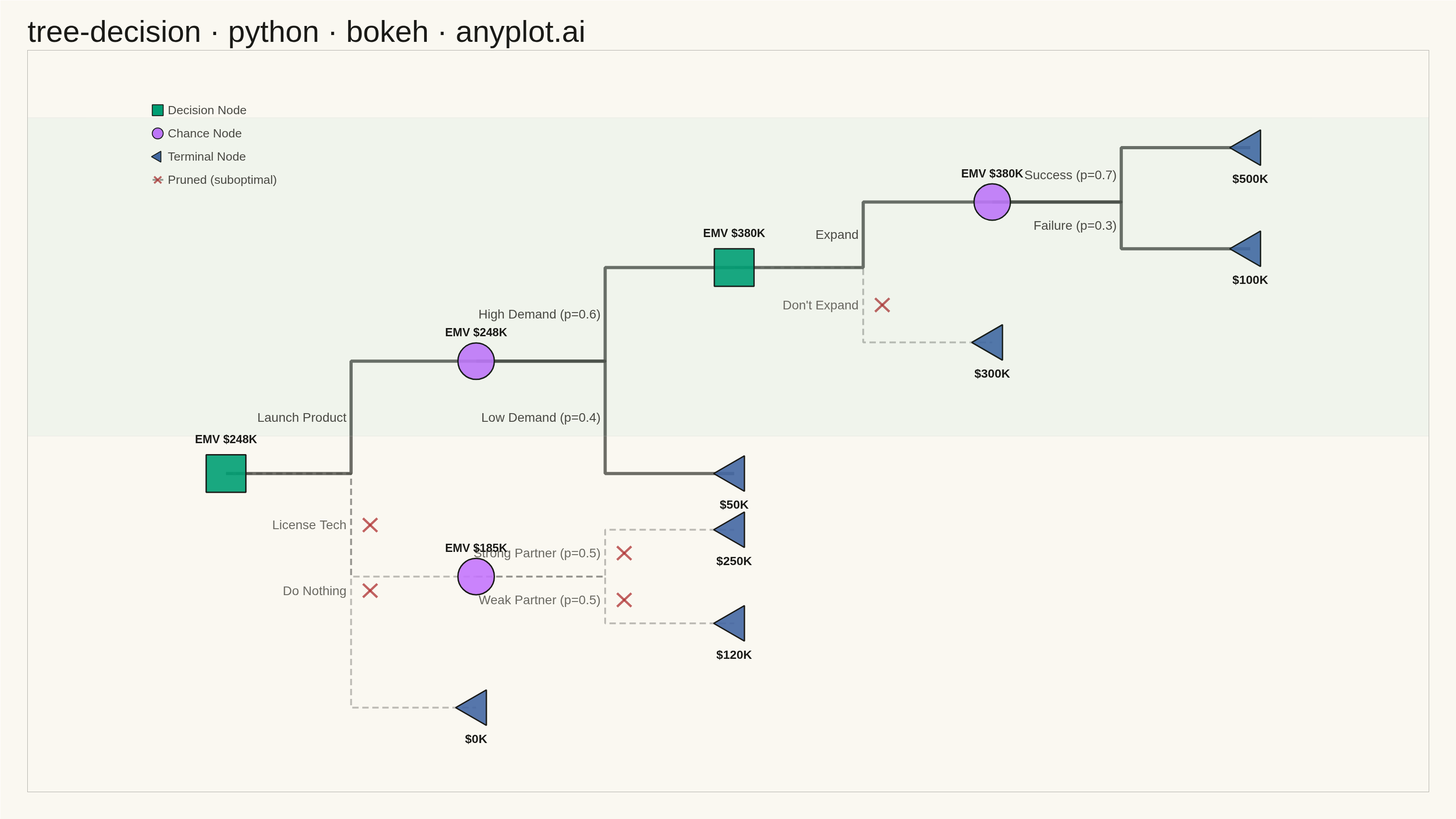
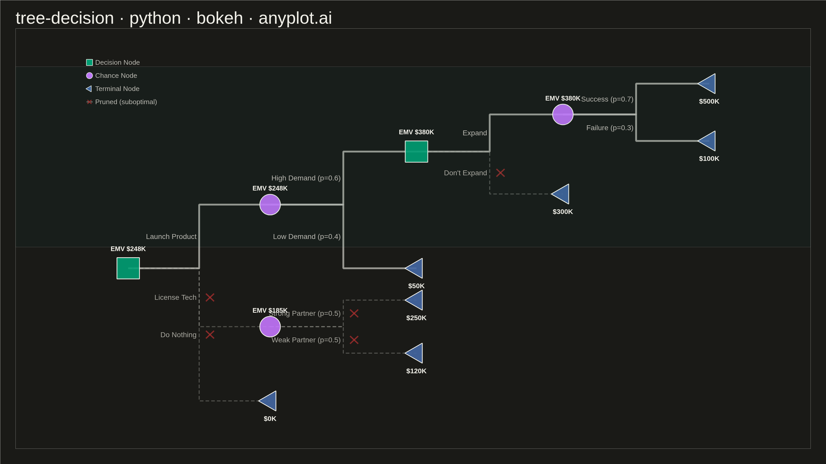
A tree-structured diagram for sequential decision analysis, displaying decision nodes (squares), chance nodes (circles), and terminal outcome nodes (triangles) connected by branching paths. Each chance branch is labeled with probabilities, terminal nodes show payoff values, and Expected Monetary Values (EMV) are calculated via rollback at each node. Rejected (pruned) branches are visually marked, making it easy to trace the optimal decision path through a multi-stage problem.
""" anyplot.ai
tree-decision: Decision Tree Visualization with Probabilities
Library: bokeh 3.9.0 | Python 3.13.13
Quality: 84/100 | Updated: 2026-06-02
"""

import os
import time
from pathlib import Path

import numpy as np
from bokeh.io import output_file, save
from bokeh.models import BoxAnnotation, ColumnDataSource, HoverTool, Label
from bokeh.plotting import figure
from selenium import webdriver
from selenium.webdriver.chrome.options import Options


THEME = os.getenv("ANYPLOT_THEME", "light")

# Theme-adaptive chrome tokens (Imprint palette)
PAGE_BG = "#FAF8F1" if THEME == "light" else "#1A1A17"
ELEVATED_BG = "#FFFDF6" if THEME == "light" else "#242420"
INK = "#1A1A17" if THEME == "light" else "#F0EFE8"
INK_SOFT = "#4A4A44" if THEME == "light" else "#B8B7B0"
INK_MUTED = "#6B6A63" if THEME == "light" else "#A8A79F"

# Imprint palette — node types in canonical order
COLOR_DECISION = "#009E73"  # position 1, brand green
COLOR_CHANCE = "#C475FD"  # position 2, lavender
COLOR_TERMINAL = "#4467A3"  # position 3, blue
COLOR_PRUNE = "#AE3030"  # position 5, semantic: error/rejected

# Data — Two-stage investment decision tree
# EMV rollback:
#   C3: 0.7*500 + 0.3*100 = 380
#   D2: max(380, 300) = 380  → Don't Expand pruned
#   C1: 0.6*380 + 0.4*50  = 248
#   C2: 0.5*250 + 0.5*120 = 185
#   D1: max(248, 185, 0)  = 248 → License & Do Nothing pruned
#
# Layout designed for 3200×1800 canvas (data units ≈ pixels at 1:1 scale).
# Columns at x ∈ {220, 850, 1500, 2150, 2800}; rows spread across y ∈ [100, 1700].
nodes = {
    "D1": {"type": "decision", "x": 220, "y": 750, "value": 248},
    "C1": {"type": "chance", "x": 850, "y": 1050, "value": 248},
    "C2": {"type": "chance", "x": 850, "y": 475, "value": 185},
    "T1": {"type": "terminal", "x": 850, "y": 125, "value": 0},
    "D2": {"type": "decision", "x": 1500, "y": 1300, "value": 380},
    "T2": {"type": "terminal", "x": 1500, "y": 750, "value": 50},
    "T3": {"type": "terminal", "x": 1500, "y": 600, "value": 250},
    "T4": {"type": "terminal", "x": 1500, "y": 350, "value": 120},
    "C3": {"type": "chance", "x": 2150, "y": 1475, "value": 380},
    "T5": {"type": "terminal", "x": 2150, "y": 1100, "value": 300},
    "T6": {"type": "terminal", "x": 2800, "y": 1620, "value": 500},
    "T7": {"type": "terminal", "x": 2800, "y": 1350, "value": 100},
}

edges = [
    ("D1", "C1", "Launch Product", None, False),
    ("D1", "C2", "License Tech", None, True),
    ("D1", "T1", "Do Nothing", None, True),
    ("C1", "D2", "High Demand", 0.6, False),
    ("C1", "T2", "Low Demand", 0.4, False),
    ("C2", "T3", "Strong Partner", 0.5, True),
    ("C2", "T4", "Weak Partner", 0.5, True),
    ("D2", "C3", "Expand", None, False),
    ("D2", "T5", "Don't Expand", None, True),
    ("C3", "T6", "Success", 0.7, False),
    ("C3", "T7", "Failure", 0.3, False),
]

# Canvas: 3200×1800 landscape (Imprint catalog standard)
W, H = 3200, 1800

p = figure(
    width=W,
    height=H,
    title="tree-decision · python · bokeh · anyplot.ai",
    x_range=(-280, 3250),
    y_range=(-100, 1880),
    toolbar_location=None,  # omit toolbar so exported PNG height == H
    min_border_bottom=60,
    min_border_left=60,
    min_border_top=110,
    min_border_right=60,
)

# Subtle fill highlighting the optimal-path region (upper portion)
p.add_layout(BoxAnnotation(bottom=850, top=1700, fill_color=COLOR_DECISION, fill_alpha=0.04))

# Draw edges: right-angle connectors (horizontal → vertical → horizontal)
for src, dst, label, prob, pruned in edges:
    sx, sy = nodes[src]["x"], nodes[src]["y"]
    dx, dy = nodes[dst]["x"], nodes[dst]["y"]
    mid_x = (sx + dx) / 2

    lw = 4 if pruned else 7
    alpha = 0.35 if pruned else 0.80
    dash = [14, 8] if pruned else "solid"

    p.line(
        [sx, mid_x, mid_x, dx], [sy, sy, dy, dy], line_width=lw, line_alpha=alpha, line_color=INK_SOFT, line_dash=dash
    )

    # Branch label — placed on the vertical connector segment
    branch_text = f"{label} (p={prob})" if prob is not None else label
    label_y = (sy + dy) / 2
    p.add_layout(
        Label(
            x=mid_x,
            y=label_y,
            text=branch_text,
            text_font_size="21pt",
            text_color=INK_MUTED if pruned else INK_SOFT,
            text_align="right",
            text_baseline="middle",
            x_offset=-10,
        )
    )

    # Red cross mark on pruned branches
    if pruned:
        cx, cy, cs = mid_x + 48, label_y, 18
        p.multi_line(
            [[cx - cs, cx + cs], [cx - cs, cx + cs]],
            [[cy - cs, cy + cs], [cy + cs, cy - cs]],
            line_width=5,
            line_color=COLOR_PRUNE,
            line_alpha=0.75,
        )

# Build ColumnDataSources for each node type
decision_nodes = {k: v for k, v in nodes.items() if v["type"] == "decision"}
chance_nodes = {k: v for k, v in nodes.items() if v["type"] == "chance"}
terminal_nodes = {k: v for k, v in nodes.items() if v["type"] == "terminal"}


decision_src = ColumnDataSource(
    data={
        "x": [n["x"] for n in decision_nodes.values()],
        "y": [n["y"] for n in decision_nodes.values()],
        "name": list(decision_nodes.keys()),
        "emv": [f"${n['value']}K" for n in decision_nodes.values()],
        "node_type": ["Decision"] * len(decision_nodes),
    }
)
chance_src = ColumnDataSource(
    data={
        "x": [n["x"] for n in chance_nodes.values()],
        "y": [n["y"] for n in chance_nodes.values()],
        "name": list(chance_nodes.keys()),
        "emv": [f"${n['value']}K" for n in chance_nodes.values()],
        "node_type": ["Chance"] * len(chance_nodes),
    }
)
terminal_src = ColumnDataSource(
    data={
        "x": [n["x"] for n in terminal_nodes.values()],
        "y": [n["y"] for n in terminal_nodes.values()],
        "name": list(terminal_nodes.keys()),
        "emv": [f"${n['value']}K" for n in terminal_nodes.values()],
        "node_type": ["Terminal"] * len(terminal_nodes),
    }
)

# Decision nodes — squares (width/height in data units ≈ pixels)
r_dec = p.rect(
    "x",
    "y",
    width=100,
    height=100,
    source=decision_src,
    fill_color=COLOR_DECISION,
    fill_alpha=0.90,
    line_color=INK,
    line_width=3,
)

# Chance nodes — circles (size in screen px)
r_ch = p.scatter(
    "x",
    "y",
    source=chance_src,
    size=80,
    marker="circle",
    fill_color=COLOR_CHANCE,
    fill_alpha=0.90,
    line_color=INK,
    line_width=3,
)

# Terminal nodes — right-pointing triangles (larger than predecessor)
r_term = p.scatter(
    "x",
    "y",
    source=terminal_src,
    size=78,
    marker="triangle",
    fill_color=COLOR_TERMINAL,
    fill_alpha=0.90,
    line_color=INK,
    line_width=3,
    angle=np.pi / 2,
)

# Interactive hover
p.add_tools(
    HoverTool(
        renderers=[r_dec, r_ch, r_term],
        tooltips=f"""
        <div style="font-size:18px;padding:8px;background:{ELEVATED_BG};
                    color:{INK};border-radius:4px;border:1px solid {INK_SOFT};">
            <b>@name</b> (@node_type)<br/>Value: <b>@emv</b>
        </div>
        """,
        point_policy="snap_to_data",
    )
)

# Node labels — placed in data coordinates to avoid overlapping node shapes.
# Decision/chance: label bottom 70–75 data units above node centre (clears shape top).
# Terminal: label top 65 data units below node centre (clears triangle bottom).
for _nid, nd in nodes.items():
    if nd["type"] == "terminal":
        p.add_layout(
            Label(
                x=nd["x"],
                y=nd["y"] - 65,  # below triangle
                text=f"${nd['value']}K",
                text_font_size="20pt",
                text_font_style="bold",
                text_align="center",
                text_baseline="top",
                text_color=INK,
            )
        )
    else:
        # Square half-height = 50 data units → label bottom at y+75 clears top edge
        offset = 75 if nd["type"] == "decision" else 60
        p.add_layout(
            Label(
                x=nd["x"],
                y=nd["y"] + offset,
                text=f"EMV ${nd['value']}K",
                text_font_size="19pt",
                text_font_style="bold",
                text_align="center",
                text_baseline="bottom",
                text_color=INK,
            )
        )

# Legend — top-left corner
leg_x = 30
leg_y0 = 1720
leg_gap = 62

for i, (ntype, color, marker, label) in enumerate(
    [
        ("decision", COLOR_DECISION, "square", "Decision Node"),
        ("chance", COLOR_CHANCE, "circle", "Chance Node"),
        ("terminal", COLOR_TERMINAL, "triangle", "Terminal Node"),
    ]
):
    ly = leg_y0 - i * leg_gap
    angle = np.pi / 2 if ntype == "terminal" else 0
    p.scatter([leg_x + 18], [ly], size=24, marker=marker, fill_color=color, line_color=INK, line_width=2, angle=angle)
    p.add_layout(
        Label(
            x=leg_x + 18,
            y=ly,
            text=label,
            text_font_size="20pt",
            text_color=INK_SOFT,
            x_offset=22,
            text_baseline="middle",
        )
    )

# Pruned legend entry
ly = leg_y0 - 3 * leg_gap
p.line([leg_x + 5, leg_x + 32], [ly, ly], line_width=4, line_dash=[10, 6], line_color=INK_SOFT, line_alpha=0.55)
cs = 9
p.multi_line(
    [[leg_x + 18 - cs, leg_x + 18 + cs], [leg_x + 18 - cs, leg_x + 18 + cs]],
    [[ly - cs, ly + cs], [ly + cs, ly - cs]],
    line_width=4,
    line_color=COLOR_PRUNE,
    line_alpha=0.75,
)
p.add_layout(
    Label(
        x=leg_x + 18,
        y=ly,
        text="Pruned (suboptimal)",
        text_font_size="20pt",
        text_color=INK_SOFT,
        x_offset=22,
        text_baseline="middle",
    )
)

# Theme-adaptive chrome
p.title.text_font_size = "50pt"
p.title.text_font_style = "normal"
p.title.text_color = INK
p.xaxis.visible = False
p.yaxis.visible = False
p.xgrid.visible = False
p.ygrid.visible = False
p.outline_line_color = INK_SOFT
p.outline_line_alpha = 0.25
p.background_fill_color = PAGE_BG
p.border_fill_color = PAGE_BG

# Save interactive HTML (required catalog artifact)
output_file(f"plot-{THEME}.html")
save(p)

# Screenshot via headless Chrome — same pattern as highcharts.py.
# window-size must match figure width/height exactly so the bokeh canvas fills
# the viewport without white space.
opts = Options()
for arg in (
    "--headless=new",
    "--no-sandbox",
    "--disable-dev-shm-usage",
    "--disable-gpu",
    f"--window-size={W},{H}",
    "--hide-scrollbars",
):
    opts.add_argument(arg)

driver = webdriver.Chrome(options=opts)
# Force exact viewport dimensions via CDP — avoids the ~139 px browser-chrome
# overhead that headless Chrome subtracts from --window-size height.
driver.execute_cdp_cmd(
    "Emulation.setDeviceMetricsOverride", {"width": W, "height": H, "deviceScaleFactor": 1, "mobile": False}
)
driver.get(f"file://{Path(f'plot-{THEME}.html').resolve()}")
time.sleep(3)  # let bokeh JS render
driver.save_screenshot(f"plot-{THEME}.png")
driver.quit()
Runnable source as JSON, for any HTTP client: https://api.anyplot.ai/specs/tree-decision/bokeh/code. Any spec id and library id listed in llms-full.txt fit the same URL shape; every URL below is complete and callable.
{
  "spec_id": "tree-decision",
  "language": "python",
  "library": "bokeh",
  "page": "https://anyplot.ai/tree-decision/python/bokeh",
  "hub": "https://anyplot.ai/tree-decision",
  "code_json": "https://api.anyplot.ai/specs/tree-decision/bokeh/code",
  "spec_json": "https://api.anyplot.ai/specs/tree-decision",
  "render_light_png": "https://storage.googleapis.com/anyplot-images/plots/tree-decision/python/bokeh/plot-light.png",
  "render_dark_png": "https://storage.googleapis.com/anyplot-images/plots/tree-decision/python/bokeh/plot-dark.png",
  "interactive_light_html": "https://storage.googleapis.com/anyplot-images/plots/tree-decision/python/bokeh/plot-light.html",
  "interactive_dark_html": "https://storage.googleapis.com/anyplot-images/plots/tree-decision/python/bokeh/plot-dark.html",
  "quality_score": 84.0,
  "license": "MIT",
  "guide": "https://anyplot.ai/llms.txt"
}
Part of Decision Tree Visualization with Probabilities on anyplot.ai.