The same plot in 14 other libraries — Python: Altair, Bokeh, lets-plot, Matplotlib, Plotly, plotnine, Pygal, Seaborn; Julia: Makie.jl; JavaScript: Chart.js, D3.js, Apache ECharts, Highcharts, MUI X Charts. Compare all 15 side by side: Decision Tree Visualization with Probabilities in Python, R, Julia and JavaScript.
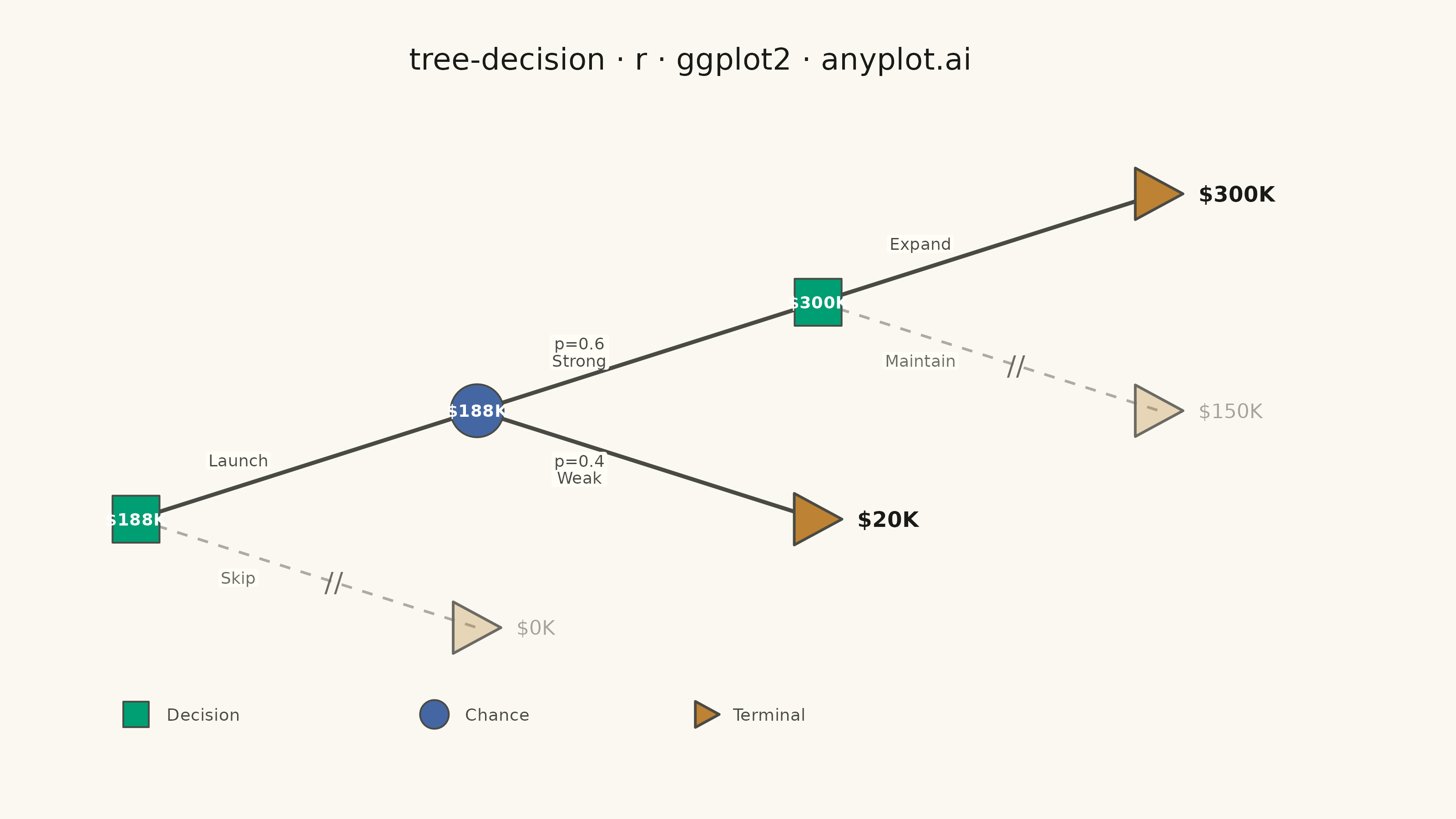
A tree-structured diagram for sequential decision analysis, displaying decision nodes (squares), chance nodes (circles), and terminal outcome nodes (triangles) connected by branching paths. Each chance branch is labeled with probabilities, terminal nodes show payoff values, and Expected Monetary Values (EMV) are calculated via rollback at each node. Rejected (pruned) branches are visually marked, making it easy to trace the optimal decision path through a multi-stage problem.
#' anyplot.ai
#' tree-decision: Decision Tree Visualization with Probabilities
#' Library: ggplot2 3.5.1 | R 4.4.1
#' Quality: 90/100 | Created: 2026-06-02

library(ggplot2)
library(ragg)

set.seed(42)

# Theme tokens (Imprint palette)
THEME       <- Sys.getenv("ANYPLOT_THEME", "light")
PAGE_BG     <- if (THEME == "light") "#FAF8F1" else "#1A1A17"
ELEVATED_BG <- if (THEME == "light") "#FFFDF6" else "#242420"
INK         <- if (THEME == "light") "#1A1A17" else "#F0EFE8"
INK_SOFT    <- if (THEME == "light") "#4A4A44" else "#B8B7B0"
INK_MUTED   <- if (THEME == "light") "#6B6A63" else "#A8A79F"

# Imprint palette positions used
COL_DEC  <- "#009E73"  # position 1 — decision nodes (brand green)
COL_CHC  <- "#4467A3"  # position 3 — chance nodes (blue)
COL_TERM <- "#BD8233"  # position 4 — terminal nodes (ochre)

# Tech startup product launch decision tree
# Stage 1: Launch vs. Skip
# Stage 2 (if Launch): Market Strong (p=0.6) vs. Weak (p=0.4)
# Stage 3 (if Strong): Expand vs. Maintain
#
# EMV rollback:
#   EMV(D1) = max($300K Expand, $150K Maintain) = $300K  -> Expand wins
#   EMV(C0) = 0.6 * $300K + 0.4 * $20K = $188K
#   EMV(D0) = max($188K Launch, $0 Skip) = $188K          -> Launch wins

nodes <- data.frame(
  id      = c("D0",    "C0",    "D1",    "T1",  "T2",    "T3",  "T4"),
  type    = c("dec",   "chc",   "dec",   "term","term",  "term","term"),
  x       = c(1.0,     3.0,     5.0,     7.0,   7.0,     5.0,   3.0),
  y       = c(0.0,     0.5,     1.0,     1.5,   0.5,     0.0,  -0.5),
  emv_lbl = c("$188K", "$188K", "$300K", NA,    NA,      NA,    NA),
  payoff  = c(NA,      NA,      NA,      300,   150,     20,    0),
  pruned  = c(FALSE,   FALSE,   FALSE,   FALSE, TRUE,    FALSE, TRUE),
  stringsAsFactors = FALSE
)

edges <- data.frame(
  from   = c("D0",    "D0",   "C0",           "C0",          "D1",     "D1"),
  to     = c("C0",    "T4",   "D1",           "T3",          "T1",     "T2"),
  label  = c("Launch","Skip", "p=0.6\nStrong","p=0.4\nWeak", "Expand", "Maintain"),
  pruned = c(FALSE,   TRUE,   FALSE,          FALSE,         FALSE,    TRUE),
  stringsAsFactors = FALSE
)

# Attach node coordinates to edges
fi       <- match(edges$from, nodes$id)
ti       <- match(edges$to,   nodes$id)
edges$x0 <- nodes$x[fi];  edges$y0 <- nodes$y[fi]
edges$x1 <- nodes$x[ti];  edges$y1 <- nodes$y[ti]

# Branch label at 30% from source; offset above/below line depending on slope
edges$lx <- edges$x0 + 0.30 * (edges$x1 - edges$x0)
edges$ly <- edges$y0 + 0.30 * (edges$y1 - edges$y0)
edges$dy <- ifelse(edges$y1 >= edges$y0, 0.12, -0.12)

# Pruned-mark position at 58% from source
edges$px <- edges$x0 + 0.58 * (edges$x1 - edges$x0)
edges$py <- edges$y0 + 0.58 * (edges$y1 - edges$y0)

# Right-pointing triangle polygons for terminal nodes
hw <- 0.14
term_rows <- which(nodes$type == "term")
tri_frames <- lapply(seq_along(term_rows), function(i) {
  ni <- term_rows[i]
  data.frame(
    x      = c(nodes$x[ni] - hw, nodes$x[ni] - hw, nodes$x[ni] + hw),
    y      = c(nodes$y[ni] - hw * 0.85, nodes$y[ni] + hw * 0.85, nodes$y[ni]),
    pruned = nodes$pruned[ni],
    grp    = i
  )
})
tri_data <- do.call(rbind, tri_frames)

# Subsets for conditional styling
e_live  <- edges[!edges$pruned, ]
e_dead  <- edges[edges$pruned, ]
t_live  <- tri_data[!tri_data$pruned, ]
t_dead  <- tri_data[tri_data$pruned, ]
n_dec   <- nodes[nodes$type == "dec", ]
n_chc   <- nodes[nodes$type == "chc", ]
n_emv   <- nodes[!is.na(nodes$emv_lbl), ]
n_paylv <- nodes[nodes$type == "term" & !nodes$pruned, ]
n_paydt <- nodes[nodes$type == "term" &  nodes$pruned, ]

p <- ggplot() +
  # Edges: active
  geom_segment(
    data = e_live,
    aes(x = x0, y = y0, xend = x1, yend = y1),
    color = INK_SOFT, linewidth = 0.75
  ) +
  # Edges: pruned (dashed, muted)
  geom_segment(
    data = e_dead,
    aes(x = x0, y = y0, xend = x1, yend = y1),
    color = INK_MUTED, linewidth = 0.5, linetype = "dashed", alpha = 0.55
  ) +
  # Terminal triangles: active
  geom_polygon(
    data = t_live,
    aes(x = x, y = y, group = grp),
    fill = COL_TERM, color = INK_SOFT
  ) +
  # Terminal triangles: pruned (faded)
  geom_polygon(
    data = t_dead,
    aes(x = x, y = y, group = grp),
    fill = COL_TERM, color = INK_MUTED, alpha = 0.30
  ) +
  # Chance nodes (circles)
  geom_point(
    data = n_chc,
    aes(x = x, y = y),
    shape = 21, size = 9.5, fill = COL_CHC, color = INK_SOFT, stroke = 0.5
  ) +
  # Decision nodes (squares)
  geom_point(
    data = n_dec,
    aes(x = x, y = y),
    shape = 22, size = 9.5, fill = COL_DEC, color = INK_SOFT, stroke = 0.5
  ) +
  # EMV values inside decision/chance nodes
  geom_text(
    data = n_emv,
    aes(x = x, y = y, label = emv_lbl),
    color = "white", size = 2.4, fontface = "bold"
  ) +
  # Branch labels: active
  geom_label(
    data = e_live,
    aes(x = lx, y = ly + dy, label = label),
    color = INK_SOFT, fill = ELEVATED_BG, size = 2.3, lineheight = 0.85,
    label.padding = unit(0.13, "lines"), label.size = 0
  ) +
  # Branch labels: pruned
  geom_label(
    data = e_dead,
    aes(x = lx, y = ly + dy, label = label),
    color = INK_MUTED, fill = ELEVATED_BG, size = 2.3, lineheight = 0.85,
    label.padding = unit(0.13, "lines"), label.size = 0
  ) +
  # Double-strike pruned mark
  geom_text(
    data = e_dead,
    aes(x = px, y = py),
    label = "//", color = INK_MUTED, size = 3.8
  ) +
  # Payoff labels: active terminals (right of triangle)
  geom_text(
    data = n_paylv,
    aes(x = x + hw + 0.09, y = y, label = paste0("$", payoff, "K")),
    color = INK, size = 3.0, fontface = "bold", hjust = 0
  ) +
  # Payoff labels: pruned terminals
  geom_text(
    data = n_paydt,
    aes(x = x + hw + 0.09, y = y, label = paste0("$", payoff, "K")),
    color = INK_MUTED, size = 2.8, hjust = 0, alpha = 0.6
  ) +
  # Legend: Decision node
  annotate("point", x = 1.0, y = -0.90, shape = 22, size = 5,
           fill = COL_DEC, color = INK_SOFT) +
  annotate("text", x = 1.18, y = -0.90, label = "Decision",
           hjust = 0, size = 2.4, color = INK_SOFT) +
  # Legend: Chance node
  annotate("point", x = 2.75, y = -0.90, shape = 21, size = 5,
           fill = COL_CHC, color = INK_SOFT) +
  annotate("text", x = 2.93, y = -0.90, label = "Chance",
           hjust = 0, size = 2.4, color = INK_SOFT) +
  # Legend: Terminal node (small right-pointing triangle)
  annotate("polygon",
           x = c(4.35 - 0.07, 4.35 - 0.07, 4.35 + 0.07),
           y = c(-0.90 - 0.06, -0.90 + 0.06, -0.90),
           fill = COL_TERM, color = INK_SOFT) +
  annotate("text", x = 4.50, y = -0.90, label = "Terminal",
           hjust = 0, size = 2.4, color = INK_SOFT) +
  coord_cartesian(xlim = c(0.35, 8.15), ylim = c(-1.15, 1.95), expand = FALSE) +
  labs(title = "tree-decision · r · ggplot2 · anyplot.ai") +
  theme_void() +
  theme(
    plot.background  = element_rect(fill = PAGE_BG, color = PAGE_BG),
    panel.background = element_rect(fill = PAGE_BG, color = NA),
    plot.title       = element_text(
      color = INK, size = 12, hjust = 0.5,
      margin = margin(t = 14, b = 8)
    ),
    plot.margin = margin(t = 5, r = 40, b = 20, l = 10)
  )

ggsave(
  filename = sprintf("plot-%s.png", THEME),
  plot     = p,
  device   = ragg::agg_png,
  width    = 8,
  height   = 4.5,
  units    = "in",
  dpi      = 400
)
Runnable source as JSON, for any HTTP client: https://api.anyplot.ai/specs/tree-decision/ggplot2/code. Any spec id and library id listed in llms-full.txt fit the same URL shape; every URL below is complete and callable.
{
  "spec_id": "tree-decision",
  "language": "r",
  "library": "ggplot2",
  "page": "https://anyplot.ai/tree-decision/r/ggplot2",
  "hub": "https://anyplot.ai/tree-decision",
  "code_json": "https://api.anyplot.ai/specs/tree-decision/ggplot2/code",
  "spec_json": "https://api.anyplot.ai/specs/tree-decision",
  "render_light_png": "https://storage.googleapis.com/anyplot-images/plots/tree-decision/r/ggplot2/plot-light.png",
  "render_dark_png": "https://storage.googleapis.com/anyplot-images/plots/tree-decision/r/ggplot2/plot-dark.png",
  "quality_score": 90.0,
  "license": "MIT",
  "guide": "https://anyplot.ai/llms.txt"
}
Part of Decision Tree Visualization with Probabilities on anyplot.ai.